Example of modeling relational data in DynamoDB

This example describes how to model relational data in Amazon DynamoDB. A DynamoDB table design corresponds to the relational order entry schema that is shown in Relational modeling. It follows the Adjacency list design pattern, which is a common way to represent relational data structures in DynamoDB.

The design pattern requires you to define a set of entity types that usually correlate to the various tables in the relational schema. Entity items are then added to the table using a compound (partition and sort) primary key. The partition key of these entity items is the attribute that uniquely identifies the item and is referred to generically on all items as PK. The sort key attribute contains an attribute value that you can use for an inverted index or global secondary index. It is generically referred to as SK.

You define the following entities, which support the relational order entry schema.

1. HR-Employee - PK: EmployeeID, SK: Employee Name

2. HR-Region - PK: RegionID, SK: Region Name

3. HR-Country - PK: CountryId, SK: Country Name

4. HR-Location - PK: LocationID, SK: Country Name

5. HR-Job - PK: JobID, SK: Job Title

6. HR-Department - PK: DepartmentID, SK: DepartmentID

7. OE-Customer - PK: CustomerID, SK: AccountRepID

8. OE-Order - PK OrderID, SK: CustomerID

9. OE-Product - PK: ProductID, SK: Product Name

10. OE-Warehouse - PK: WarehouseID, SK: Region Name

After adding these entity items to the table, you can define the relationships between them by adding edge items to the entity item partitions. The following table demonstrates this step.

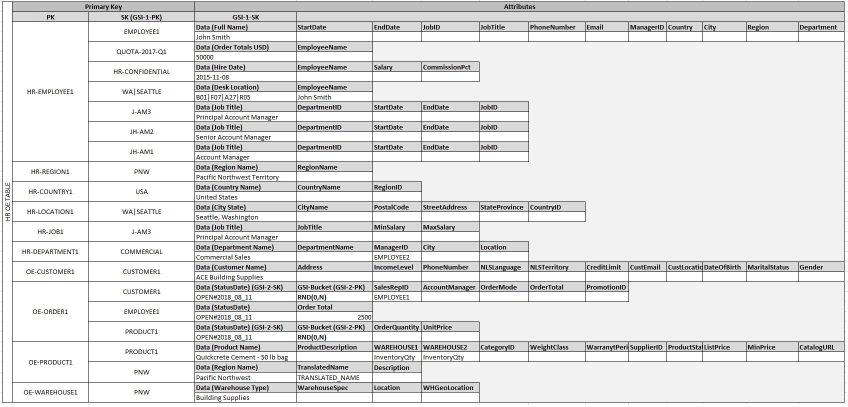
In this example, the Employee, Order, and Product Entity partitions on the table have additional edge items that contain pointers to other entity items on the table. Next, define a few global secondary indexes (GSIs) to support all the access patterns defined previously. The entity items don't all use the same type of value for the primary key or the sort key attribute. All that is required is to have the primary key and sort key attributes present to be inserted on the table.

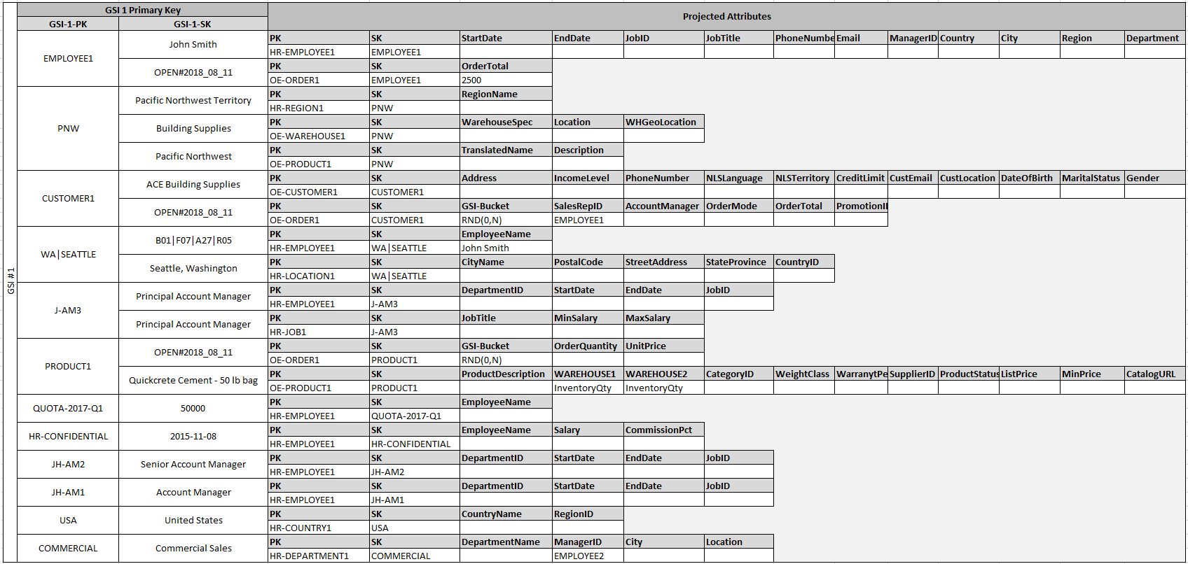
The fact that some of these entities use proper names and others use other entity IDs as sort key values allows the same global secondary index to support multiple types of queries. This technique is called GSI overloading. It effectively eliminates the default limit of 20 global secondary indexes for tables that contain multiple item types. This is shown in the following diagram as GSI 1.

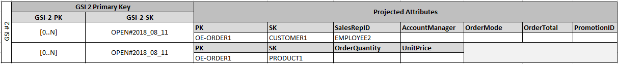
GSI 2 is designed to support a fairly common application access pattern, which is to get all the items on the table that have a certain state. For a large table with an uneven distribution of items across available states, this access pattern can result in a hot key, unless the items are distributed across more than one logical partition that can be queried in parallel. This design pattern is called write sharding.

To accomplish this for GSI 2, the application adds the GSI 2 primary key attribute to every Order item. It populates that with a random number in a range of 0–N, where N can generically be calculated using the following formula, unless there is a specific reason to do otherwise.

ItemsPerRCU = 4KB / AvgItemSize

PartitionMaxReadRate = 3K * ItemsPerRCU

N = MaxRequiredIO / PartitionMaxReadRate

For example, assume that you expect the following:

• Up to 2 million orders will be in the system, growing to 3 million in 5 years.

• Up to 20 percent of these orders will be in an OPEN state at any given time.

• The average order record is around 100 bytes, with three OrderItem records in the order partition that are around 50 bytes each, giving you an average order entity size of 250 bytes.

For that table, the N factor calculation would look like the following.

ItemsPerRCU = 4KB / 250B = 16

PartitionMaxReadRate = 3K * 16 = 48K

N = (0.2 * 3M) / 48K = 13

In this case, you need to distribute all the orders across at least 13 logical partitions on GSI 2 to ensure that a read of all Order items with an OPEN status doesn't cause a hot partition on the physical storage layer. It is a good practice to pad this number to allow for anomalies in the dataset. So a model using N = 15 is probably fine. As mentioned earlier, you do this by adding the random 0–N value to the GSI 2 PK attribute of each Order and OrderItem record that is inserted on the table.

This breakdown assumes that the access pattern that requires gathering all OPEN invoices occurs relatively infrequently so that you can use burst capacity to fulfill the request. You can query the following global secondary index using a State and Date Range Sort Key condition to produce a subset or all Orders in a given state as needed.

In this example, the items are randomly distributed across the 15 logical partitions. This structure works because the access pattern requires a large number of items to be retrieved. Therefore, it's unlikely that any of the 15 threads will return empty result sets that could potentially represent wasted capacity. A query always uses 1 read capacity unit (RCU) or 1 write capacity unit (WCU), even if nothing is returned or no data is written.

If the access pattern requires a high velocity query on this global secondary index that returns a sparse result set, it's probably better to use a hash algorithm to distribute the items rather than a random pattern. In this case, you might select an attribute that is known when the query is run at runtime and hash that attribute into a 0–14 key space when the items are inserted. Then they can be efficiently read from the global secondary index.

Finally, you can revisit the access patterns that were defined earlier. Following is the list of access patterns and the query conditions that you will use with the new DynamoDB version of the application to accommodate them.

	Access patterns	Query conditions
1	Look up Employee Details by Employee ID	Primary Key on table, ID="HR-EMPLOYEE"
2	Query Employee Details by Employee Name	Use GSI-1, PK="Employee Name"
3	Get an employee's current job details only	Primary Key on table, PK=HR-EMPLOYEE-1, SK starts with "JH"
4	Get Orders for a customer for a date range	Use GSI-1, PK=CUSTOMER1, SK="STATUS-DATE", for each StatusCode
5	Show all Orders in OPEN status for a date range across all customers	Use GSI-2, PK=query in parallel for the range [0..N], SK between OPEN-Date1 and OPEN-Date2
6	All Employees hired recently	Use GSI-1, PK="HR-CONFIDENTIAL', SK > date1
7	Find all Employees in specific Warehouse	Use GSI-1, PK=WAREHOUSE1
8	Get all Orderitems for a Product including warehouse location inventories	Use GSI-1, PK=PRODUCT1
9	Get customers by Account Rep	Use GSI-1, PK=ACCOUNT-REP
10	Get orders by Account Rep and date	Use GSI-1, PK=ACCOUNT-REP, SK="STATUS-DATE", for each StatusCode
11	Get all employees with specific Job Title	Use GSI-1, PK=JOBTITLE
12	Get inventory by Product and Warehouse	Primary Key on table, PK=OE-PRODUCT1,SK=PRODUCT1
13	Get total product inventory	Primary Key on table, PK=OE-PRODUCT1,SK=PRODUCT1
14	Get Account Reps ranked by Order Total and Sales Period	Use GSI-1, PK=YYYY-Q1, scanIndexForward=False