Performance efficiency pillar

The performance efficiency pillar of the AWS Well-Architected Framework focuses on how to optimize performance while ingesting or querying data. Performance optimization is an incremental and continual process of the following:

• Confirming business requirements

• Measuring workload performance

• Identifying under-performing components

• Tuning components to meet your business needs

The performance efficiency pillar provides use case-specific guidelines that can help you identify the right graph data model and query languages to use. It also includes best practices to follow when ingesting data into, and consuming data from, Neptune Analytics.

The performance efficiency pillar focuses on the following key areas:

• Graph modeling

• Query optimization

• Graph right-sizing

• Write optimization

Understand graph modeling for analytics

The guide Applying the AWS Well-Architected Framework for Amazon Neptune discusses graph modeling for performance efficiency. Modeling decisions that affect performance include choosing which nodes and edges are required, their IDs, their labels and properties, the direction of edges, whether labels should be generic or specific, and generally how efficiently the query engine can navigate the graph to process common queries.

These considerations apply to Neptune Analytics, too; however, it is important to distinguish between transactional and analytical usage patterns. A graph model that is efficient for queries in a transactional database such as a Neptune database might need to be reshaped for analytics.

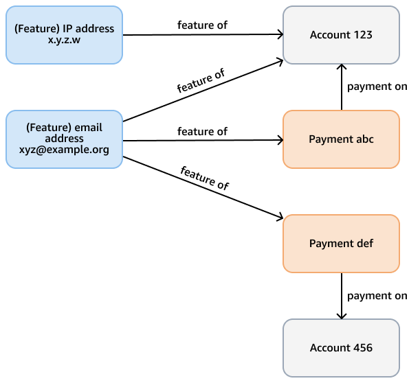
For example, consider a fraud graph in a Neptune database whose purpose is to check for fraudulent patterns in credit card payments. This graph might have nodes that represent accounts, payments, and features (such as email address, IP address, phone number) of both the account and the payment. This connected graph supports queries such as traversing a variable-length path that starts from a given payment and takes several hops to find related features and accounts. The following figure shows such a graph.

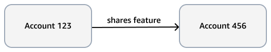
The analytical requirement might be more specific, such as finding communities of accounts that are linked by a feature. You can use the weakly connected components (WCC) algorithm for this purpose. To run it against the model in the previous example is inefficient, because it needs to traverse through several different types of nodes and edges. The model in the next diagram is more efficient. It links account nodes with a shares feature edge if the accounts themselves—or payments from the accounts—share a feature. For example, Account 123 has email feature [e-mail], and Account 456 uses that same email for a payment (Payment def).

The computational complexity of WCC is O(|E|logD), where |E| is the number of edges in the graph, and D is the diameter (the length of the longest path) that connects nodes. Because the transactional model omits inessential nodes and edges, it optimizes both the number of edges and the diameter, and reduces the WCC algorithm's complexity.

When you use Neptune Analytics, work back from required algorithms and analytical queries. If necessary, reshape the model to optimize these queries. You can reshape the model before you load data into the graph, or write queries that modify existing data in the graph.

Optimize queries

Follow these recommendations to optimize Neptune Analytics queries:

• Use parameterized queries and the query plan cache, which is enabled by default. When you use the plan cache, the engine prepares the query for later use—provided that the query completes in 100 milliseconds or less—which saves time on subsequent invocations.

• For slow queries, run an explain plan to spot bottlenecks and make improvements accordingly.

• If you use vector similarity search, decide if smaller embeddings yield accurate similarity results. You can create, store, and search smaller embeddings more efficiently.

• Follow documented best practices for using openCypher in Neptune Analytics. For example, use flattened maps in an UNWIND clause and specify edge labels where possible.

• When you use a graph algorithm, understand the algorithm's inputs and outputs, its computational complexity, and broadly how it works.

  • Before you call a graph algorithm, use a MATCH clause to minimize the input node set. For example, to limit nodes to do breadth-first search (BFS) from, follow the examples provided in the Neptune Analytics documentation.

  • Filter on node and edge labels if possible. For example, BFS has input parameters to filter traversal to a specific node label (vertexLabel) or specific edge labels (edgeLabels).

  • Use bounding parameters such as maxDepth to limit results.

  • Experiment with the concurrency parameter. Try it with a value of 0, which uses all available algorithm threads to parallelize processing. Compare that with single-threaded execution by setting the parameter to 1. An algorithm can complete faster in a single thread, especially on smaller inputs such as shallow breadth-first searches where parallelism offers no measurable reduction in execution time and might introduce overhead.

  • Choose between similar types of algorithms. For example, Bellman-Ford and delta-stepping are both single-source shortest path algorithms. When testing with your own dataset, try both algorithms and compare the results. Delta-stepping is often faster than Bellman-Ford because of its lower computational complexity. However, performance depends on the dataset and input parameters, particularly the delta parameter.

Optimize writes

Follow these practices to optimize write operations in Neptune Analytics:

• Seek the most efficient way to load data into a graph. When you load from data in Amazon S3, use bulk import if the data is greater than 50 GB in size. For smaller data, use batch load. If you get out-of-memory errors when you run batch load, consider increasing the m-NCU value or splitting the load into multiple requests. One way to accomplish this is to split files across multiple prefixes in the S3 bucket. In that case, call batch load separately for each prefix.

• Use bulk import or the batch loader to populate the initial set of graph data. Use transactional openCypher create, update, and delete operations for small changes only.

• Use either bulk import or the batch loader with a concurrency of 1 (single threaded) to ingest embeddings into the graph. Try to load embeddings up front by using one of these methods.

• Assess the dimension of vector embeddings needed for accurate similarity search in vector similarity search algorithms. Use a smaller dimension if possible. This results in faster load speed for embeddings.

• Use mutate algorithms to remember algorithmic results if required. For example, the degree mutate centrality algorithm finds the degree of each input node and writes that value as a property of the node. If the connections surrounding those nodes do not subsequently change, the property holds the correct result. There is no need to run the algorithm again.

• Use the graph reset administrative action to clear all nodes, edges, and embeddings if you need to start over. Dropping all nodes, edges, and embeddings by using an openCypher query is not feasible if your graph is large. A single drop query on a large dataset can time out. As size increases, the dataset takes longer to remove and transaction size increases. By contrast, the time to complete a graph reset is roughly constant, and the action provides the option to create a snapshot before you run it.

Right-size graphs

Overall performance depends on the provisioned capacity of a Neptune Analytics graph. Capacity is measured in units called memory-optimized Neptune Capacity Units (m-NCUs). Make sure that your graph is sufficiently sized to support your graph size and queries. Note that increased capacity doesn't necessarily improve the performance of an individual query.

If possible, create the graph by importing data from an existing source such as Amazon S3 or an existing Neptune cluster or snapshot. You can place bounds on mininum and maximum capacity. You can also change provisioned capacity on an existing graph.

Monitor CloudWatch metrics such as NumQueuedRequestsPerSec, NumOpenCypherRequestsPerSec, GraphStorageUsagePercent, GraphSizeBytes, and CPUUtilization to assess whether the graph is right-sized. Determine if more capacity is needed to support your graph size and load. For more information about how to interpret some of these metrics, see the Operational excellence pillar section.