Amazon Redshift will no longer support the creation of new Python UDFs starting November 1, 2025.
If you would like to use Python UDFs, create the UDFs prior to that date.
Existing Python UDFs will continue to function as normal. For more information, see the
blog post
Visualizing query results
After you run a query and the results display, you can turn on Chart to display a graphic visualization of the current page of results. You can use the following controls to define the content, structure, and appearance of your chart:
-
 Trace
Trace -
Represents a set of related graphical marks in a chart. You can define multiple traces in a chart.
- Type
-
You can define the trace type to represent data as one of the following:
-
Scatter chart for a scatter plot or bubble chart.
-
Bar chart to represent categories of data with vertical or horizontal bars.
-
Area chart to define filled areas.
-
Histogram that uses bars to represent frequency distribution.
-
Pie chart for a circular representation of data where each slice represents a percentage of the whole.
-
Funnel or Funnel Area chart to represent data through various stages of a process.
-
OHLC (open-high-low-close) chart often used for financial data to represent open, high, low, and close values along the x-axis, which usually represents intervals of time.
-
Candlestick chart to represent a range of values for a category over a timeline.
-
Waterfall chart to represent how an initial value increases or decreases through a series of intermediate values. Values can represent time intervals or categories.
-
Line chart to represent changes in value over time.
-
- X axis
-
You specify a table column that contains values to plot along the X axis. Columns that contain descriptive values usually represent dimensional data. Columns that contain quantitative values usually represent factual data.
- Y axis
-
You specify a table column that contains values to plot along the Y axis. Columns that contain descriptive values usually represent dimensional data. Columns that contain quantitative values usually represent factual data.
- Subplots
-
You can define additional presentations of chart data.
- Transforms
-
You can define transforms to filter trace data. You use a split transform to display multiple traces from a single source trace. You use an aggregate transform to present a trace as an average or minimum. You use a sort transform to sort a trace.
- General appearance
-
You can set defaults for background color, margin color, color scales to design palettes, text style and sizes, title style and size, and mode bar. You can define interactions for drag, click, and hover. You can define meta text. You can define default appearances for traces, axes, legends, and annotations.
To create a chart
-
Run a query and get results.
-
Turn on Charts.
-
Choose Trace and start to visualize your data.
-
Choose a chart style from one of the following:
-
Scatter
-
Bar
-
Area
-
Histogram
-
Pie
-
Funnel
-
Funnel Area
-
OHLC (open-high-low-close)
-
Candlestick
-
Waterfall
-
Line
-
-
Choose Style to customize the appearance, including colors, axes, legend, and annotations. You can add text, shapes, and images.
-
Choose Annotations to add text, shapes, and images.
-
Choose Refresh to update the chart display. Choose Full screen to expand the chart display.
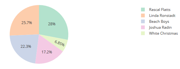
Example: Create a pie chart to visualize query results
The following example uses the Sales table of the sample database. For more information, see Sample database in the Amazon Redshift Database Developer Guide.
Following is the query that you run to provide the data for the pie chart.
select top 5 eventname, count(salesid) totalorders, sum(pricepaid) totalsales
from sales, event
where sales.eventid=event.eventid group by eventname
order by 3;
To create a pie chart for the top event by total sales
-
Run the query.
-
In the query results area, turn on Chart.
-
Choose Trace.
-
For Type, choose Pie.
-
For Values, choose totalsales.
-
For Labels, choose eventname.
-
Choose Style and then General.
-
Under Colorscales, choose Categorical and then Pastel2.
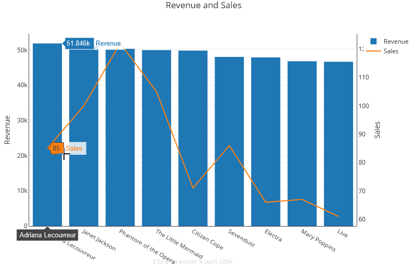
Example: Create a combination chart for comparing revenue and sales
Perform the steps in this example to create a chart that combines a bar chart for revenue data and a line graph for sales data. The following example uses the Sales table of the tickit sample database. For more information, see Sample database in the Amazon Redshift Database Developer Guide.
Following is the query that you run to provide the data for the chart.
select eventname, total_price, total_qty_sold
from  (select eventid, total_price, total_qty_sold, ntile(1000) over(order by total_price desc) as percentile
       from (select eventid, sum(pricepaid) total_price, sum(qtysold) total_qty_sold
             from   tickit.sales
             group by eventid)) Q, tickit.event E
       where Q.eventid = E.eventid
       and percentile = 1
order by total_price desc;
To create a combination chart for comparing revenue and sales
-
Run the query.
-
In the query results area, turn on Chart.
-
Under trace o, for Type, choose Bar.
-
For X, choose eventname.
-
For Y, choose total_price.
The bar chart displays with event names along the X axis.
-
Under Style, choose Traces.
-
For Name, enter Revenue.
-
Under Style, choose Axes.
-
For Titles, choose Y and enter Revenue.
The label Revenue displays on the left Y axis.
-
Under Structure, choose Traces.
-
Choose
Trace.The trace 1 options display.
-
For Type, choose Line.
-
For X, choose eventname.
-
For Y, choose total_qty_sold.
-
Under Axes To Use, for Y Axis choose
. The Y Axis displays Y2.
-
Under Style, choose Axes.
-
Under Titles, choose Y2.
-
For Name, enter Sales.
-
Under Lines, choose Y:Sales.
-
Under Axis Line, choose Show and for Position, choose Right.
Demo: Build visualizations using Amazon Redshift query editor v2
For a demo of how to build visualizations, watch the following video.
