本文為英文版的機器翻譯版本,如內容有任何歧義或不一致之處,概以英文版為準。
最佳化隨機播放
join() 和 等特定操作groupByKey()需要 Spark 執行隨機播放。隨機播放是 Spark 重新分配資料的機制,因此在 RDD 分割區之間會以不同的方式分組。隨機播放有助於修復效能瓶頸。不過,由於隨機切換通常涉及在 Spark 執行器之間複製資料,因此隨機切換是複雜且昂貴的操作。例如,隨機播放會產生下列成本:
-
磁碟輸入/輸出:
-
在磁碟上產生大量中繼檔案。
-
-
網路輸入/輸出:
-
需要許多網路連線 (連線數目 =
Mapper × Reducer)。 -
由於記錄會彙總到可能託管在不同 Spark 執行器上的新 RDD 分割區,因此您資料集的很大一部分可能會在 Spark 執行器之間透過網路移動。
-
-
CPU 和記憶體負載:
-
排序值並合併資料集。這些操作是在執行器上規劃的,對執行器造成繁重負載。
-
Shuffle 是 Spark 應用程式效能降低的最重要因素之一。儲存中繼資料時,可能會耗盡執行器本機磁碟上的空間,這會導致 Spark 任務失敗。
您可以在 CloudWatch 指標和 Spark UI 中評估隨機播放效能。
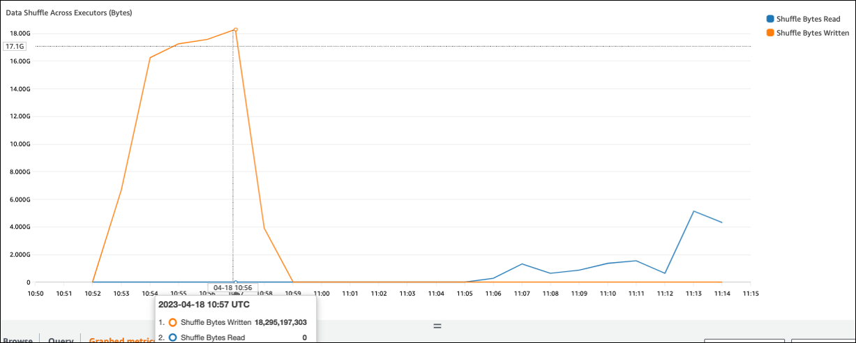
CloudWatch 指標
如果與隨機位元組讀取相比,隨機位元組寫入值很高,則 Spark 任務可能會使用隨機播放操作join()或 groupByKey()。
Spark UI
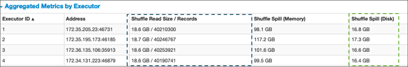
在 Spark UI 的階段索引標籤上,您可以檢查隨機讀取大小/記錄值。您也可以在執行器索引標籤上查看。
在下列螢幕擷取畫面中,每個執行器會使用隨機播放程序交換大約 18.6GB/4020000 的記錄,以交換大約 75 GB 的總隨機播放讀取大小)。
Shuffle 溢出 (磁碟) 欄顯示大量資料溢出記憶體到磁碟,這可能會導致磁碟完整或效能問題。
如果您觀察到這些症狀,而且相較於效能目標,階段需要花太久的時間,或者失敗並出現 Out Of Memory或 No space left on device錯誤,請考慮下列解決方案。
最佳化聯結
結合資料表的 join()操作是最常使用的隨機播放操作,但通常是效能瓶頸。由於加入是一項昂貴的操作,因此建議您不要使用它,除非它對您的業務需求至關重要。詢問下列問題,再次檢查您是否有效使用資料管道:
-
您是否正在重新計算也可以在其他任務中執行的聯結,以便重複使用?
-
您是否加入 ,將外部索引鍵解析為輸出的取用者未使用的值?
在您確認加入操作對於您的業務需求至關重要之後,請參閱下列選項,以符合您需求的方式最佳化您的加入。
加入前使用下推
在執行聯結之前,篩選掉 DataFrame 中不必要的資料列和資料欄。這具有下列優點:
-
減少隨機播放期間的資料傳輸量
-
減少 Spark 執行器中的處理量
-
減少資料掃描量
# Default
df_joined  = df1.join(df2, ["product_id"])

# Use Pushdown
df1_select = df1.select("product_id","product_title","star_rating").filter(col("star_rating")>=4.0)
df2_select = df2.select("product_id","category_id")
df_joined  = df1_select.join(df2_select, ["product_id"])
使用 DataFrame 聯結
嘗試使用 Spark 高階 APIdyf.toDF()。如 Apache Spark 章節中的關鍵主題所述,這些聯結操作會在內部利用 Catalyst 最佳化工具的查詢最佳化。
隨機播放和廣播雜湊聯結和提示
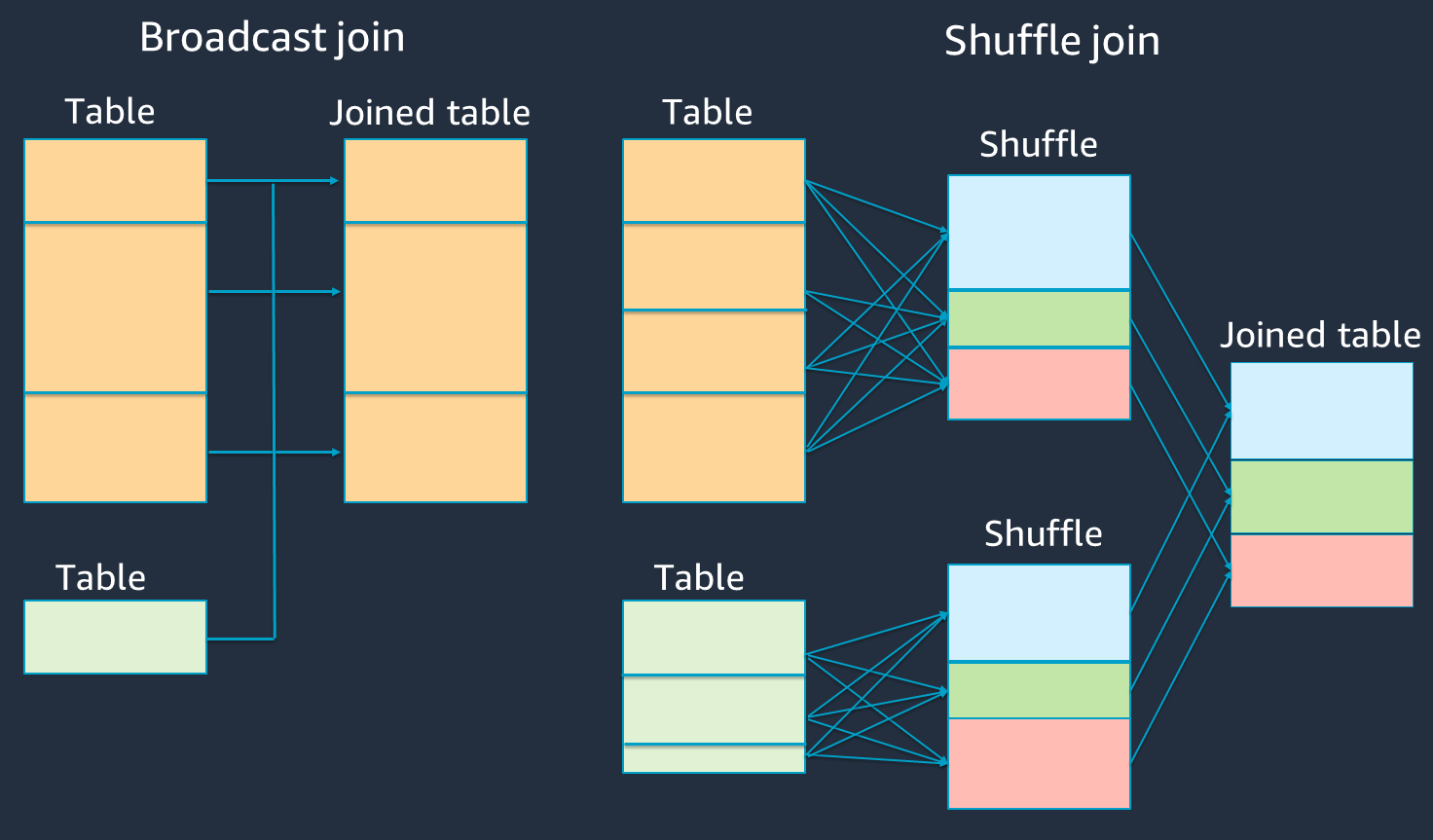
Spark 支援兩種類型的聯結:隨機聯結和廣播雜湊聯結。廣播雜湊聯結不需要隨機播放,而且比隨機播放聯結需要更少的處理。不過,它僅適用於將小型資料表加入大型資料表時。加入可放入單一 Spark 執行器記憶體的資料表時,請考慮使用廣播雜湊聯結。
下圖顯示廣播雜湊聯結和隨機聯結的高階結構和步驟。
每個聯結的詳細資訊如下所示:
-
隨機聯結:
-
隨機雜湊聯結會聯結兩個資料表,而不會排序和分配兩個資料表之間的聯結。它適用於可存放在 Spark 執行器記憶體中的小型資料表聯結。
-
排序合併聯結會分配要依索引鍵聯結的兩個資料表,並在聯結前進行排序。它適用於大型資料表的聯結。
-
-
廣播雜湊聯結:
-
廣播雜湊聯結會將較小的 RDD 或資料表推送到每個工作者節點。然後,它會執行映射端與較大 RDD 或資料表的每個分割區結合。
當您的其中一個 RDDs或資料表可以容納在記憶體中或可以容納在記憶體中時,它適用於聯結。可能的話,進行廣播雜湊聯結是有利的,因為它不需要隨機播放。您可以使用聯結提示,從 Spark 請求廣播聯結,如下所示。
# DataFrame from pySpark.sql.functions import broadcast df_joined= df_big.join(broadcast(df_small), right_df[key] == left_df[key], how='inner') -- SparkSQL SELECT /*+ BROADCAST(t1) / FROM t1 INNER JOIN t2 ON t1.key = t2.key;如需聯結提示的詳細資訊,請參閱聯結提示
。
-
在 AWS Glue 3.0 和更新版本中,您可以透過啟用自適應查詢執行
在 AWS Glue 3.0 中,您可以透過設定 來啟用自適應查詢執行。 spark.sql.adaptive.enabled=true根據預設,AWS Glue 4.0 中會啟用自適應查詢執行。
您可以設定與隨機播放和廣播雜湊聯結相關的其他參數:
-
spark.sql.adaptive.localShuffleReader.enabled -
spark.sql.adaptive.autoBroadcastJoinThreshold
如需相關參數的詳細資訊,請參閱將排序合併聯結轉換為廣播聯結
在 AWS Glue 3.0 和更新版本中,您可以使用其他聯結提示進行隨機播放來調整您的行為。
-- Join Hints for shuffle sort merge join
SELECT /*+ SHUFFLE_MERGE(t1) /  FROM t1 INNER JOIN t2 ON t1.key = t2.key;
SELECT /*+ MERGEJOIN(t2) /  FROM t1 INNER JOIN t2 ON t1.key = t2.key;
SELECT /*+ MERGE(t1) /  FROM t1 INNER JOIN t2 ON t1.key = t2.key;

-- Join Hints for shuffle hash join
SELECT /*+ SHUFFLE_HASH(t1) /  FROM t1 INNER JOIN t2 ON t1.key = t2.key;

-- Join Hints for shuffle-and-replicate nested loop join
SELECT /*+ SHUFFLE_REPLICATE_NL(t1) /  FROM t1 INNER JOIN t2 ON t1.key = t2.key;
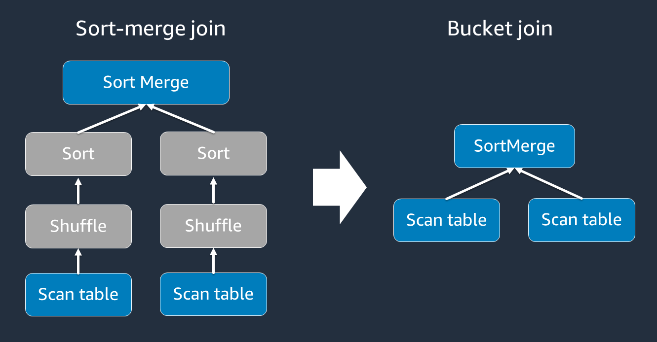
使用儲存貯體
排序合併聯結需要兩個階段,即隨機排序和排序,然後合併。這兩個階段可能會使 Spark 執行器超載,並導致 OOM 和效能問題,因為有些執行器正在合併,而其他執行器正在同時排序。在這種情況下,可以使用儲存貯體
儲存貯體資料表適用於下列項目:
-
經常透過相同金鑰加入的資料,例如
account_id -
載入每日累積資料表,例如可在一般資料欄上儲存的基底和差異資料表
您可以使用下列程式碼建立儲存貯體資料表。
df.write.bucketBy(50, "account_id").sortBy("age").saveAsTable("bucketed_table")
加入前在聯結金鑰上重新分割 DataFrames
若要在聯結前重新分割聯結金鑰上的兩個 DataFrames,請使用下列陳述式。
df1_repartitioned = df1.repartition(N,"join_key")
df2_repartitioned = df2.repartition(N,"join_key")
df_joined  = df1_repartitioned.join(df2_repartitioned,"product_id")
這將在聯結金鑰上分割兩個 (仍為個別) RDDs,然後再啟動聯結。如果兩個 RDDs具有相同分割程式碼的相同金鑰上進行分割,則 RDD 會記錄您計劃聯結在一起的 RDD,在隨機切換聯結之前,有很高的可能性會位於相同的工作者上。這可以透過減少聯結期間的網路活動和資料扭曲來改善效能。
克服資料扭曲
資料扭曲是 Spark 任務瓶頸的最常見原因之一。當資料未平均分佈於 RDD 分割區時,就會發生此狀況。這會導致該分割區的任務花費比其他分割區長得多,因而延遲應用程式的整體處理時間。
若要識別資料扭曲,請在 Spark UI 中評估下列指標:
-
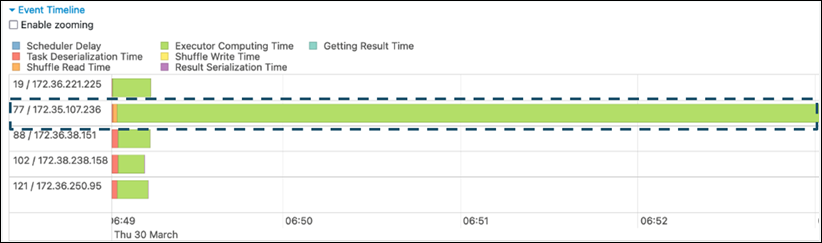
在 Spark UI 中的階段索引標籤上,檢查事件時間表頁面。您可以在下列螢幕擷取畫面中看到任務分佈不平均。分佈不均勻或執行時間過長的任務可能表示資料扭曲。
-
另一個重要的頁面是摘要指標,顯示 Spark 任務的統計資料。下列螢幕擷取畫面顯示持續時間、GC 時間、溢出 (記憶體)、溢出 (磁碟) 等的百分位數指標。
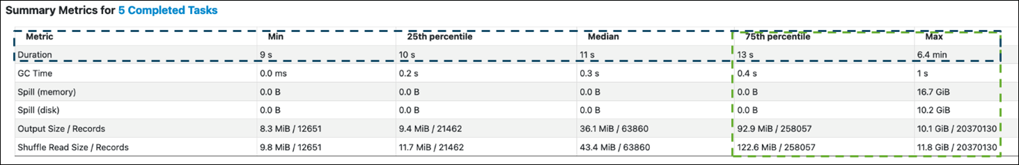
當任務平均分佈時,您會在所有百分位數中看到類似的數字。當資料扭曲時,您會在每個百分位數看到非常偏差的值。在此範例中,任務持續時間在最小值、第 25 個百分位數、中位數和第 75 個百分位數中少於 13 秒。雖然 Max 任務處理的資料是第 75 個百分位數的 100 倍,但其 6.4 分鐘的持續時間約為 30 倍。這表示至少有一個任務 (或高達 25% 的任務) 花費比其餘任務長得多。
如果您看到資料扭曲,請嘗試下列動作:
-
如果您使用 AWS Glue 3.0,請設定 來啟用自適應查詢執行。
spark.sql.adaptive.enabled=true自適應查詢執行預設為在 AWS Glue 4.0 中啟用。您也可以透過設定下列相關參數,將自適應查詢執行用於聯結引入的資料偏移:
-
spark.sql.adaptive.skewJoin.skewedPartitionFactor -
spark.sql.adaptive.skewJoin.skewedPartitionThresholdInBytes -
spark.sql.adaptive.advisoryPartitionSizeInBytes=128m (128 mebibytes or larger should be good) -
spark.sql.adaptive.coalescePartitions.enabled=true (when
                                        you want to coalesce partitions)
如需詳細資訊,請參閱 Apache Spark 文件
。 -
-
針對聯結金鑰使用具有大量值的金鑰。在隨機聯結中,系統會針對金鑰的每個雜湊值來決定分割區。如果聯結索引鍵的基數太低,雜湊函數更有可能在跨分割區分散資料時執行不良任務。因此,如果您的應用程式和商業邏輯支援它,請考慮使用較高的基數索引鍵或複合索引鍵。
# Use Single Primary Key
df_joined = df1_select.join(df2_select, ["primary_key"])

# Use Composite Key
df_joined = df1_select.join(df2_select, ["primary_key","secondary_key"])
使用快取
當您使用重複DataFrames時,請使用 或 df.persist()將計算結果快取到每個 Spark 執行器的記憶體和磁碟上,以避免額外的隨機處理df.cache()或運算。Spark 也支援在磁碟上保留 RDDs 或跨多個節點複寫 (儲存層級
例如,您可以透過新增 來保留 DataFrames df.persist() 當不再需要快取時,您可以使用 unpersist 來捨棄快取的資料。
df = spark.read.parquet("s3://<Bucket>/parquet/product_category=Books/")
df_high_rate = df.filter(col("star_rating")>=4.0)
df_high_rate.persist()

df_joined1 = df_high_rate.join(<Table1>, ["key"])
df_joined2 = df_high_rate.join(<Table2>, ["key"])
df_joined3 = df_high_rate.join(<Table3>, ["key"])
...
df_high_rate.unpersist()
移除不需要的 Spark 動作
避免執行不必要的動作,例如 count、 show 或 collect。如 Apache Spark 章節中的關鍵主題所述,Spark 很慢。每次在 RDD 上執行動作時,可能會重新計算每個轉換的 RDD。當您使用許多 Spark 動作時,會呼叫每個動作的多個來源存取、任務計算和隨機執行。
如果您在商業環境中不需要 collect() 或其他動作,請考慮移除這些動作。
注意
盡可能避免collect()在商業環境中使用 Spark。collect() 動作會將 Spark 執行器中計算的所有結果傳回 Spark 驅動程式,這可能會導致 Spark 驅動程式傳回 OOM 錯誤。為了避免 OOM 錯誤,Spark spark.driver.maxResultSize = 1GB 預設會設定 ,將傳回 Spark 驅動程式的資料大小上限限制為 1 GB。
