Le traduzioni sono generate tramite traduzione automatica. In caso di conflitto tra il contenuto di una traduzione e la versione originale in Inglese, quest'ultima prevarrà.
Utilizzo di EXPLAIN e EXPLAIN ANALYZE in Athena
L'istruzione EXPLAIN mostra il piano di esecuzione logico o distribuito di un'istruzione SQL specificata o convalida l'istruzione SQL. È possibile generare i risultati in formato testo o in formato dati per il rendering in un grafico.
Nota
È possibile visualizzare rappresentazioni grafiche di piani logici e distribuiti per le proprie query nella console Athena senza utilizzare la sintassi EXPLAIN. Per ulteriori informazioni, consulta Visualizza i piani di esecuzione per le query SQL.
L'istruzione EXPLAIN ANALYZE mostra sia il piano di esecuzione distribuito di un'istruzione SQL specificata che il costo computazionale di ciascuna operazione in una query SQL. È possibile eseguire l'output dei risultati in formato testo o JSON.
Considerazioni e limitazioni
Le istruzioni EXPLAIN e EXPLAIN ANALYZE in Athena hanno le seguenti limitazioni.
-
Poiché le query
EXPLAINnon scansionano alcun dato, Athena non addebita alcun costo per loro. Tuttavia, poiché le queryEXPLAINeffettuano chiamate a AWS Glue per recuperare i metadati della tabella, potresti ricevere addebiti da Glue se le chiamate superano il limite del piano gratuito per Glue. -
Poiché vengono eseguite le query
EXPLAIN ANALYZE, viene eseguita la scansione dei dati e Athena addebita la quantità di dati scansionati. -
Le informazioni sul filtraggio di righe o celle definite in Lake Formation e le informazioni sulle statistiche delle query non vengono visualizzate nell'output di
EXPLAINeEXPLAIN ANALYZE.
Sintassi EXPLAIN
EXPLAIN [ (option[, ...]) ]statement
optionIl valore di può essere uno dei seguenti:
FORMAT { TEXT | GRAPHVIZ | JSON }
TYPE { LOGICAL | DISTRIBUTED | VALIDATE | IO }
Se l'opzione FORMAT non è specificata, l'output avrà il formato di default TEXT. Il IO tipo fornisce informazioni sulle tabelle e sugli schemi letti dalla query.
Sintassi EXPLAIN ANALYZE
Oltre all'output incluso in EXPLAIN, l'output EXPLAIN
ANALYZE include anche statistiche del runtime per la query specificata, ad esempio l'utilizzo della CPU, l'input del numero di righe e l'output del numero di righe.
EXPLAIN ANALYZE [ (option[, ...]) ]statement
optionIl valore di può essere uno dei seguenti:
FORMAT { TEXT | JSON }
Se l'opzione FORMAT non è specificata, l'output avrà il formato di default TEXT. Perché tutte le query per EXPLAIN ANALYZE sono DISTRIBUTED, l'opzione TYPE non è disponibile per EXPLAIN ANALYZE.
statementIl valore di può essere uno dei seguenti:
SELECT
CREATE TABLE AS SELECT
INSERT
UNLOAD
Esempi di EXPLAIN
Gli esempi seguenti per l'avanzamento di EXPLAIN vanno dai più semplici ai più complessi.
Nell'esempio seguente, EXPLAIN mostra il piano di esecuzione per una query SELECT nei log di Elastic Load Balancing. Il formato viene impostato per impostazione predefinita sull'output di testo.
EXPLAIN
SELECT
   request_timestamp,
   elb_name,
   request_ip
FROM sampledb.elb_logs;
Risultati
- Output[request_timestamp, elb_name, request_ip] => [[request_timestamp, elb_name, request_ip]]
    - RemoteExchange[GATHER] => [[request_timestamp, elb_name, request_ip]]
        - TableScan[awsdatacatalog:HiveTableHandle{schemaName=sampledb, tableName=elb_logs,
analyzePartitionValues=Optional.empty}] => [[request_timestamp, elb_name, request_ip]]
                LAYOUT: sampledb.elb_logs
                request_ip := request_ip:string:2:REGULAR
                request_timestamp := request_timestamp:string:0:REGULAR
                elb_name := elb_name:string:1:REGULAR
Puoi usare la console Athena per eseguire un grafico su un piano di query. Inserisci un'istruzione SELECT come la seguente nell'editor di query, quindi seleziona Run (Esegui).
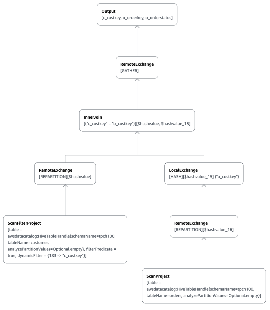
SELECT
      c.c_custkey,
      o.o_orderkey,
      o.o_orderstatus
   FROM tpch100.customer c
   JOIN tpch100.orders o
       ON c.c_custkey = o.o_custkey
La pagina Explain dell'editor di query Athena si apre e mostra un piano distribuito e un piano logico per la query. Il seguente grafico mostra il piano logico per l'esempio.
Importante
Attualmente, alcuni filtri di partizione potrebbero non essere visibili nel grafico ad albero degli operatori annidato anche se Athena li applica alla tua query. Per verificare l'effetto di tali filtri, esegui EXPLAIN o EXPLAIN
ANALYZE sulla query e visualizza i risultati.
Per ulteriori informazioni sull'utilizzo delle funzionalità grafiche del piano di query nella console Athena, consulta Visualizza i piani di esecuzione per le query SQL.
Quando si utilizza un predicato di filtro in una chiave partizionata per eseguire una query su una tabella partizionata, il motore di query applica il predicato alla chiave partizionata per ridurre la quantità di dati letti.
Nell'esempio seguente viene utilizzato una query EXPLAIN per verificare la cesura delle partizioni per una query SELECT su una tabella partizionata. Innanzitutto, un'istruzione CREATE TABLEcrea la tabella tpch100.orders_partitioned. La tabella è partizionata sulla colonna o_orderdate.
CREATE TABLE `tpch100.orders_partitioned`( `o_orderkey` int, `o_custkey` int, `o_orderstatus` string, `o_totalprice` double, `o_orderpriority` string, `o_clerk` string, `o_shippriority` int, `o_comment` string) PARTITIONED BY ( `o_orderdate` string) ROW FORMAT SERDE 'org.apache.hadoop.hive.ql.io.parquet.serde.ParquetHiveSerDe' STORED AS INPUTFORMAT 'org.apache.hadoop.hive.ql.io.parquet.MapredParquetInputFormat' OUTPUTFORMAT 'org.apache.hadoop.hive.ql.io.parquet.MapredParquetOutputFormat' LOCATION 's3://amzn-s3-demo-bucket/<your_directory_path>/'
La tabella tpch100.orders_partitioned ha diverse partizioni su o_orderdate, come mostrato dal comando SHOW PARTITIONS.
SHOW PARTITIONS tpch100.orders_partitioned; o_orderdate=1994 o_orderdate=2015 o_orderdate=1998 o_orderdate=1995 o_orderdate=1993 o_orderdate=1997 o_orderdate=1992 o_orderdate=1996
La seguente query EXPLAIN verifica la cesura delle partizioni sull'istruzione SELECTspecificata.
EXPLAIN SELECT o_orderkey, o_custkey, o_orderdate FROM tpch100.orders_partitioned WHERE o_orderdate = '1995'
Risultati
Query Plan
- Output[o_orderkey, o_custkey, o_orderdate] => [[o_orderkey, o_custkey, o_orderdate]]
- RemoteExchange[GATHER] => [[o_orderkey, o_custkey, o_orderdate]]
- TableScan[awsdatacatalog:HiveTableHandle{schemaName=tpch100, tableName=orders_partitioned,
analyzePartitionValues=Optional.empty}] => [[o_orderkey, o_custkey, o_orderdate]]
LAYOUT: tpch100.orders_partitioned
o_orderdate := o_orderdate:string:-1:PARTITION_KEY
:: [[1995]]
o_custkey := o_custkey:int:1:REGULAR
o_orderkey := o_orderkey:int:0:REGULARIl testo in grassetto nel risultato mostra che il predicato o_orderdate =
'1995' è stato applicato su PARTITION_KEY.
La seguente query EXPLAIN verifica l'ordine di join e il tipo di join dell'istruzione SELECT. Utilizzare una query come questa per esaminare l'utilizzo della memoria della query in modo da ridurre le possibilità di ottenere un errore EXCEEDED_LOCAL_MEMORY_LIMIT.
EXPLAIN (TYPE DISTRIBUTED) SELECT c.c_custkey, o.o_orderkey, o.o_orderstatus FROM tpch100.customer c JOIN tpch100.orders o ON c.c_custkey = o.o_custkey WHERE c.c_custkey = 123
Risultati
Query Plan
Fragment 0 [SINGLE]
Output layout: [c_custkey, o_orderkey, o_orderstatus]
Output partitioning: SINGLE []
Stage Execution Strategy: UNGROUPED_EXECUTION
- Output[c_custkey, o_orderkey, o_orderstatus] => [[c_custkey, o_orderkey, o_orderstatus]]
- RemoteSource[1] => [[c_custkey, o_orderstatus, o_orderkey]]
Fragment 1 [SOURCE]
Output layout: [c_custkey, o_orderstatus, o_orderkey]
Output partitioning: SINGLE []
Stage Execution Strategy: UNGROUPED_EXECUTION
- CrossJoin => [[c_custkey, o_orderstatus, o_orderkey]]
Distribution: REPLICATED
- ScanFilter[table = awsdatacatalog:HiveTableHandle{schemaName=tpch100,
tableName=customer, analyzePartitionValues=Optional.empty}, grouped = false,
filterPredicate = ("c_custkey" = 123)] => [[c_custkey]]
LAYOUT: tpch100.customer
c_custkey := c_custkey:int:0:REGULAR
- LocalExchange[SINGLE] () => [[o_orderstatus, o_orderkey]]
- RemoteSource[2] => [[o_orderstatus, o_orderkey]]
Fragment 2 [SOURCE]
Output layout: [o_orderstatus, o_orderkey]
Output partitioning: BROADCAST []
Stage Execution Strategy: UNGROUPED_EXECUTION
- ScanFilterProject[table = awsdatacatalog:HiveTableHandle{schemaName=tpch100,
tableName=orders, analyzePartitionValues=Optional.empty}, grouped = false,
filterPredicate = ("o_custkey" = 123)] => [[o_orderstatus, o_orderkey]]
LAYOUT: tpch100.orders
o_orderstatus := o_orderstatus:string:2:REGULAR
o_custkey := o_custkey:int:1:REGULAR
o_orderkey := o_orderkey:int:0:REGULARLa query di esempio è stata ottimizzata in un cross join per prestazioni migliori. I risultati mostrano che tpch100.orders sarà distribuito come tipo di distribuzione BROADCAST. Ciò implica che la tabella tpch100.orders verrà distribuita a tutti i nodi che eseguono l'operazione di join. Il tipo di distribuzione BROADCAST richiederà che tutti i risultati filtrati della tabella tpch100.orders siano inseriti nella memoria di ogni nodo che esegue l'operazione di join.
Tuttavia, la tabella tpch100.customer è più piccola di tpch100.orders. Poiché tpch100.customer richiede meno memoria, è possibile riscrivere la query su BROADCAST
tpch100.customer invece che su tpch100.orders. In questo modo si riduce la possibilità che la query riceva l'errore EXCEEDED_LOCAL_MEMORY_LIMIT. La strategia presuppone i seguenti punti:
-
tpch100.customer.c_custkeyè unico nella tabellatpch100.customer. -
Esiste una relazione di one-to-many mappatura tra
tpch100.customeretpch100.orders.
L'esempio seguente mostra la query riscritta.
SELECT c.c_custkey, o.o_orderkey, o.o_orderstatus FROM tpch100.orders o JOIN tpch100.customer c -- the filtered results of tpch100.customer are distributed to all nodes. ON c.c_custkey = o.o_custkey WHERE c.c_custkey = 123
Puoi utilizzare una query EXPLAIN per verificare l'efficacia dei predicati di filtraggio. È possibile utilizzare i risultati per rimuovere i predicati che non hanno alcun effetto, come nell'esempio seguente.
EXPLAIN SELECT c.c_name FROM tpch100.customer c WHERE c.c_custkey = CAST(RANDOM() * 1000 AS INT) AND c.c_custkey BETWEEN 1000 AND 2000 AND c.c_custkey = 1500
Risultati
Query Plan
- Output[c_name] => [[c_name]]
- RemoteExchange[GATHER] => [[c_name]]
- ScanFilterProject[table =
awsdatacatalog:HiveTableHandle{schemaName=tpch100,
tableName=customer, analyzePartitionValues=Optional.empty},
filterPredicate = (("c_custkey" = 1500) AND ("c_custkey" =
CAST(("random"() * 1E3) AS int)))] => [[c_name]]
LAYOUT: tpch100.customer
c_custkey := c_custkey:int:0:REGULAR
c_name := c_name:string:1:REGULARfilterPredicate nei risultati mostra che l'ottimizzatore ha unito i tre predicati originali in due predicati e ha cambiato il loro ordine di applicazione.
filterPredicate = (("c_custkey" = 1500) AND ("c_custkey" = CAST(("random"() * 1E3) AS int)))
Poiché i risultati mostrano che il predicato AND c.c_custkey BETWEEN
1000 AND 2000 non ha alcun effetto, è possibile rimuovere questo predicato senza modificare i risultati della query.
Per informazioni sui termini utilizzati nei risultati delle query EXPLAIN, consulta Comprendi i risultati della dichiarazione Athena EXPLAIN.
Esempi di EXPLAIN ANALYZE
Gli esempi seguenti mostrano query e output EXPLAIN ANALYZE di esempio.
Nell'esempio seguente, vengono EXPLAIN ANALYZE illustrati il piano di esecuzione e i costi di calcolo per una SELECT query sui CloudFront log. Il formato viene impostato per impostazione predefinita sull'output di testo.
EXPLAIN ANALYZE SELECT FROM cloudfront_logs LIMIT 10
Risultati
 Fragment 1
     CPU: 24.60ms, Input: 10 rows (1.48kB); per task: std.dev.: 0.00, Output: 10 rows (1.48kB)
     Output layout: [date, time, location, bytes, requestip, method, host, uri, status, referrer,\
       os, browser, browserversion]
Limit[10] => [[date, time, location, bytes, requestip, method, host, uri, status, referrer, os,\
  browser, browserversion]]
             CPU: 1.00ms (0.03%), Output: 10 rows (1.48kB)
             Input avg.: 10.00 rows, Input std.dev.: 0.00%
LocalExchange[SINGLE] () => [[date, time, location, bytes, requestip, method, host, uri, status, referrer, os,\
 browser, browserversion]]
                 CPU: 0.00ns (0.00%), Output: 10 rows (1.48kB)
                 Input avg.: 0.63 rows, Input std.dev.: 387.30%
RemoteSource[2] => [[date, time, location, bytes, requestip, method, host, uri, status, referrer, os,\
  browser, browserversion]]
                     CPU: 1.00ms (0.03%), Output: 10 rows (1.48kB)
                     Input avg.: 0.63 rows, Input std.dev.: 387.30%

 Fragment 2
     CPU: 3.83s, Input: 998 rows (147.21kB); per task: std.dev.: 0.00, Output: 20 rows (2.95kB)
     Output layout: [date, time, location, bytes, requestip, method, host, uri, status, referrer, os,\
       browser, browserversion]
LimitPartial[10] => [[date, time, location, bytes, requestip, method, host, uri, status, referrer, os,\
  browser, browserversion]]
             CPU: 5.00ms (0.13%), Output: 20 rows (2.95kB)
             Input avg.: 166.33 rows, Input std.dev.: 141.42%
TableScan[awsdatacatalog:HiveTableHandle{schemaName=default, tableName=cloudfront_logs,\
  analyzePartitionValues=Optional.empty},
grouped = false] => [[date, time, location, bytes, requestip, method, host, uri, st
                 CPU: 3.82s (99.82%), Output: 998 rows (147.21kB)
                 Input avg.: 166.33 rows, Input std.dev.: 141.42%
                 LAYOUT: default.cloudfront_logs
                 date := date:date:0:REGULAR
                 referrer := referrer:string:9:REGULAR
                 os := os:string:10:REGULAR
                 method := method:string:5:REGULAR
                 bytes := bytes:int:3:REGULAR
                 browser := browser:string:11:REGULAR
                 host := host:string:6:REGULAR
                 requestip := requestip:string:4:REGULAR
                 location := location:string:2:REGULAR
                 time := time:string:1:REGULAR
                 uri := uri:string:7:REGULAR
                 browserversion := browserversion:string:12:REGULAR
                 status := status:int:8:REGULAR
L'esempio seguente mostra il piano di esecuzione e i costi di calcolo per una SELECT query sui CloudFront log. L'esempio specifica JSON come formato di output.
EXPLAIN ANALYZE (FORMAT JSON) SELECT * FROM cloudfront_logs LIMIT 10
Risultati
{
    "fragments": [{
        "id": "1",

        "stageStats": {
            "totalCpuTime": "3.31ms",
            "inputRows": "10 rows",
            "inputDataSize": "1514B",
            "stdDevInputRows": "0.00",
            "outputRows": "10 rows",
            "outputDataSize": "1514B"
        },
        "outputLayout": "date, time, location, bytes, requestip, method, host,\
           uri, status, referrer, os, browser, browserversion",

        "logicalPlan": {
            "1": [{
                "name": "Limit",
                "identifier": "[10]",
                "outputs": ["date", "time", "location", "bytes", "requestip", "method", "host",\
                  "uri", "status", "referrer", "os", "browser", "browserversion"],
                "details": "",
                "distributedNodeStats": {
                    "nodeCpuTime": "0.00ns",
                    "nodeOutputRows": 10,
                    "nodeOutputDataSize": "1514B",
                    "operatorInputRowsStats": [{
                        "nodeInputRows": 10.0,
                        "nodeInputRowsStdDev": 0.0
                    }]
                },
                "children": [{
                    "name": "LocalExchange",
                    "identifier": "[SINGLE] ()",
                    "outputs": ["date", "time", "location", "bytes", "requestip", "method", "host",\
                      "uri", "status", "referrer", "os", "browser", "browserversion"],
                    "details": "",
                    "distributedNodeStats": {
                        "nodeCpuTime": "0.00ns",
                        "nodeOutputRows": 10,
                        "nodeOutputDataSize": "1514B",
                        "operatorInputRowsStats": [{
                            "nodeInputRows": 0.625,
                            "nodeInputRowsStdDev": 387.2983346207417
                        }]
                    },
                    "children": [{
                        "name": "RemoteSource",
                        "identifier": "[2]",
                        "outputs": ["date", "time", "location", "bytes", "requestip", "method", "host",\
                          "uri", "status", "referrer", "os", "browser", "browserversion"],
                        "details": "",
                        "distributedNodeStats": {
                            "nodeCpuTime": "0.00ns",
                            "nodeOutputRows": 10,
                            "nodeOutputDataSize": "1514B",
                            "operatorInputRowsStats": [{
                                "nodeInputRows": 0.625,
                                "nodeInputRowsStdDev": 387.2983346207417
                            }]
                        },
                        "children": []
                    }]
                }]
            }]
        }
    }, {
        "id": "2",

        "stageStats": {
            "totalCpuTime": "1.62s",
            "inputRows": "500 rows",
            "inputDataSize": "75564B",
            "stdDevInputRows": "0.00",
            "outputRows": "10 rows",
            "outputDataSize": "1514B"
        },
        "outputLayout": "date, time, location, bytes, requestip, method, host, uri, status,\
           referrer, os, browser, browserversion",

        "logicalPlan": {
            "1": [{
                "name": "LimitPartial",
                "identifier": "[10]",
                "outputs": ["date", "time", "location", "bytes", "requestip", "method", "host", "uri",\
                  "status", "referrer", "os", "browser", "browserversion"],
                "details": "",
                "distributedNodeStats": {
                    "nodeCpuTime": "0.00ns",
                    "nodeOutputRows": 10,
                    "nodeOutputDataSize": "1514B",
                    "operatorInputRowsStats": [{
                        "nodeInputRows": 83.33333333333333,
                        "nodeInputRowsStdDev": 223.60679774997897
                    }]
                },
                "children": [{
                    "name": "TableScan",
                    "identifier": "[awsdatacatalog:HiveTableHandle{schemaName=default,\
                       tableName=cloudfront_logs, analyzePartitionValues=Optional.empty},\
                       grouped = false]",
                    "outputs": ["date", "time", "location", "bytes", "requestip", "method", "host", "uri",\
                       "status", "referrer", "os", "browser", "browserversion"],
                    "details": "LAYOUT: default.cloudfront_logs\ndate := date:date:0:REGULAR\nreferrer :=\
                       referrer: string:9:REGULAR\nos := os:string:10:REGULAR\nmethod := method:string:5:\
                       REGULAR\nbytes := bytes:int:3:REGULAR\nbrowser := browser:string:11:REGULAR\nhost :=\
                       host:string:6:REGULAR\nrequestip := requestip:string:4:REGULAR\nlocation :=\
                       location:string:2:REGULAR\ntime := time:string:1: REGULAR\nuri := uri:string:7:\
                       REGULAR\nbrowserversion := browserversion:string:12:REGULAR\nstatus :=\
                       status:int:8:REGULAR\n",
                    "distributedNodeStats": {
                        "nodeCpuTime": "1.62s",
                        "nodeOutputRows": 500,
                        "nodeOutputDataSize": "75564B",
                        "operatorInputRowsStats": [{
                            "nodeInputRows": 83.33333333333333,
                            "nodeInputRowsStdDev": 223.60679774997897
                        }]
                    },
                    "children": []
                }]
            }]
        }
    }]
}
Risorse aggiuntive
Per ulteriori informazioni consulta le seguenti risorse.
-
Visualizza le statistiche e i dettagli di esecuzione per le query completate
-
Documentazione
EXPLAINdi Trino -
Documentazione
EXPLAIN ANALYZEdi Trino -
Ottimizzazione delle prestazioni delle query federate con EXPLAIN e EXPLAIN ANALYZE in Amazon Athena
nel Blog sui Big Data di AWS .
