Case study

This section examines a real-world business scenario and application for quantifying uncertainty in deep learning systems. Suppose you want a machine learning model to automatically judge whether a sentence is grammatically unacceptable (negative case) or acceptable (positive case). Consider the following business process: If the model flags a sentence as grammatically acceptable (positive), you process it automatically, without human review. If the model flags the sentence as unacceptable (negative), you pass the sentence to a human for review and correction. The case study uses deep ensembles along with temperature scaling.

This scenario has two business objectives:

• High recall for negative cases. We want to catch all sentences that have grammatical errors.

• Reduction of the manual workload. We want to auto-process cases that have no grammatical errors as much as possible.

Baseline results

When applying a single model to the data with no dropout at test time, these are the results:

• For positive sample: recall=94%, precision=82%

• For negative sample: recall=52%, precision=79%

The model has much lower performance for negative samples. However, for business applications, recall for negative samples should be the most important metric.

Application of deep ensembles

To quantify model uncertainty, we used the standard deviations of individual model predictions across deep ensembles. Our hypothesis is that for false positives (FP) and false negatives (FN) we expect to see the uncertainty to be much higher than for true positives (TP) and true negatives (TN). Specifically, the model should have high confidence when it is correct and low confidence when it is wrong, so we can use uncertainty to tell when to trust the model’s output.

The following confusion matrix shows the uncertainty distribution across FN, FP, TN, and TP data. The probability of negative standard deviation is the standard deviation of the probability of negatives across models. The median, mean, and standard deviations are aggregated across the dataset.

	Probability of negative standard deviation
Label	Median	Mean	Standard deviation
FN	0.061	0.060	0.027
FP	0.063	0.062	0.040
TN	0.039	0.045	0.026
TP	0.009	0.020	0.025

As the matrix shows, the model performed the best for TP, so that has the lowest uncertainty. The model performed the worst for FP, so that has the highest uncertainty, which is in line with our hypothesis.

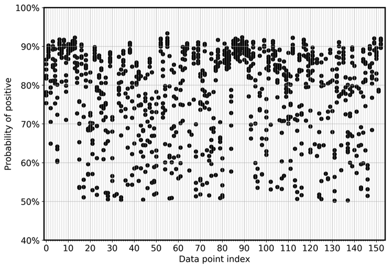
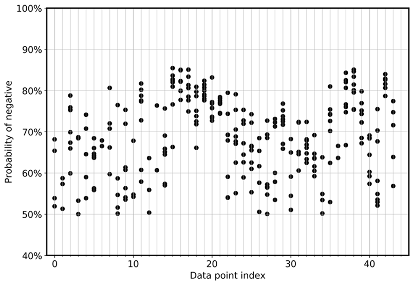
To directly visualize the model’s deviation among ensembles, the following graph plots probability in a scatter view for FN and FP for the CoLA data. Each vertical line is for one specific input sample. The graph shows eight ensemble model views. That is, each vertical line has eight data points. These points either perfectly overlap or are distributed in a range.

The first graph shows that for the FPs, the probability of being positive distributes between 0.5 and 0.925 across all eight models in the ensemble.

Similarly, the next graph shows that for the FNs, the probability of being negative distributes between 0.5 and 0.85 among the eight models in the ensemble.

Defining a decision rule

To maximize the benefit of the results, we use the following ensemble rule: For each input, we take the model that has the lowest probability of being positive (acceptable) to make flagging decisions. If the selected probability is larger than, or equal to, the threshold value, we flag the case as acceptable and auto-process it. Otherwise, we send the case for human review. This is a conservative decision rule that is appropriate in highly regulated environments.

Evaluating the results

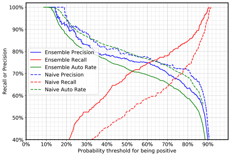
The following graph shows the precision, recall, and auto (automation) rate for the negative cases (cases with grammatical errors). The automation rate refers to the percentage of cases that will be automatically processed because the model flags the sentence as acceptable. A perfect model with 100% recall and precision would achieve a 69% (positive cases/total cases) automation rate, because only positive cases will be automatically processed.

The comparison between the deep ensemble and naïve cases shows that, for the same threshold setting, recall increases quite drastically and precision decreases slightly. (The automation rate depends on the positive and negative sample ratio in the test dataset.) For example:

• Using a threshold value of 0.5:

  • With a single model, the recall for negative cases will be 52%.

  • With the deep ensemble approach, the recall value will be 69%.

• Using a threshold value of 0.88:

  • With a single model, the recall for negative cases will be 87%.

  • With the deep ensemble approach, the recall value will be 94%.

You can see that deep ensemble can boost certain metrics (in our case, the recall of negative cases) for business applications, without a requirement to increase the size of the training data, its quality, or a change in the model’s method.