Monte Carlo dropout
One of the most popular ways to estimate uncertainty is by inferring predictive distributions with Bayesian neural networks. To denote a predictive distribution, use:

with target
 , input
 , and
, and
 many training examples
 . When you obtain a predictive distribution, you can inspect the variance and
uncover uncertainty. One way to learn a predictive distribution requires learning a distribution
over functions, or, equivalently, a distribution over the parameters (that is, the parametric
posterior distribution
. When you obtain a predictive distribution, you can inspect the variance and
uncover uncertainty. One way to learn a predictive distribution requires learning a distribution
over functions, or, equivalently, a distribution over the parameters (that is, the parametric
posterior distribution
 .
.
The Monte Carlo (MC) dropout technique (Gal and Ghahramani 2016)
provides a scalable way to learn a predictive distribution. MC dropout works by randomly
switching off neurons in a neural network, which regularizes the network. Each dropout
configuration corresponds to a different sample from the approximate parametric posterior
distribution
 :
:

where
 corresponds to a dropout configuration, or, equivalently, a simulation ~,
sampled from the approximate parametric posterior
, as shown in the following figure. Sampling from the approximate posterior
enables Monte Carlo integration of the model’s likelihood, which uncovers
the predictive distribution, as follows:
corresponds to a dropout configuration, or, equivalently, a simulation ~,
sampled from the approximate parametric posterior
, as shown in the following figure. Sampling from the approximate posterior
enables Monte Carlo integration of the model’s likelihood, which uncovers
the predictive distribution, as follows:
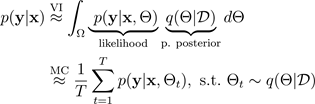
For simplicity, the likelihood may be assumed to be Gaussian distributed:

with the Gaussian function
 specified by the mean
 and variance
 parameters, which are output by simulations from the Monte Carlo dropout
BNN:
parameters, which are output by simulations from the Monte Carlo dropout
BNN:

The following figure illustrates MC dropout. Each dropout configuration yields a different output by randomly switching neurons off (gray circles) and on (black circles) with each forward propagation. Multiple forward passes with different dropout configurations yield a predictive distribution over the mean p(f(x, ø)).
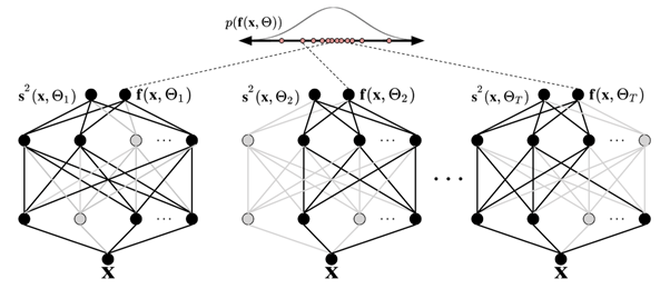
The number of forward passes through the data should be evaluated quantitatively, but 30-100 is an appropriate range to consider (Gal and Ghahramani 2016).
