Architecture components of an Amazon Redshift data warehouse
We recommend that you have a basic understanding of the core architecture components in an Amazon Redshift data warehouse. This knowledge can help you better understand how to design your queries and tables for optimal performance.
A data warehouse in Amazon Redshift consists of the following core architecture components:
-
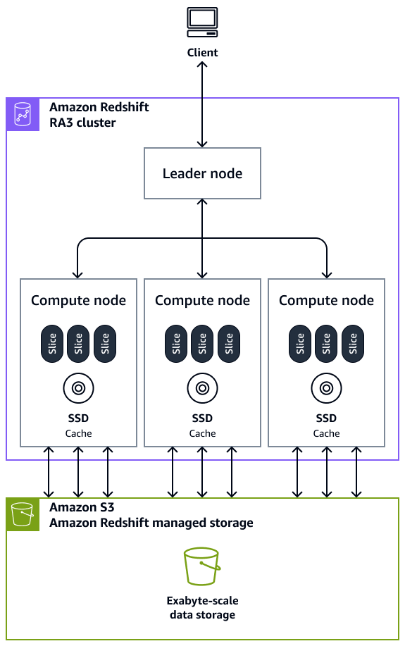
Clusters – A cluster, which is composed of one or more compute nodes, is the core infrastructure component of an Amazon Redshift data warehouse. Compute nodes are transparent to external applications, but your client application interacts directly with the leader node only. A typical cluster has two or more compute nodes. The compute nodes are coordinated through the leader node.
-
Leader node – A leader node manages the communications for client programs and all compute nodes. A leader node also prepares the plans for running a query whenever a query is submitted to a cluster. When the plans are ready, the leader node compiles code, distributes the compiled code to the compute nodes, and then assigns slices of data to each compute node to process the query results.
-
Compute node – A compute node runs a query. The leader node compiles code for individual elements of the plan to run the query and assigns the code to individual compute nodes. The compute nodes run the compiled code and send intermediate results back to the leader node for final aggregation. Each compute node has its own dedicated CPU, memory, and attached disk storage. As your workload grows, you can increase the compute capacity and storage capacity of a cluster by increasing the number of nodes, upgrading the node type, or both.
-
Node slice – A compute node is partitioned into units called slices. Every slice in a compute node is allocated a portion of the node's memory and disk space where it processes a portion of the workload assigned to the node. The slices then work in parallel to complete the operation. Data is distributed among slices on the basis of the distribution style and distribution key of a particular table. An even distribution of data makes it possible for Amazon Redshift to evenly assign workloads to slices and maximizes the benefit of parallel processing. The number of slices per compute node is decided on the basis of the type of node. For more information, see Clusters and nodes in Amazon Redshift in the Amazon Redshift documentation.
-
Massively parallel processing (MPP) – Amazon Redshift uses MPP architecture to quickly process data, even complex queries and vast amounts of data. Multiple compute nodes run the same query code on portions of data to maximize parallel processing.
-
Client application – Amazon Redshift integrates with various data loading, extract, transform, and load (ETL), business intelligence (BI) reporting, data mining, and analytics tools. All client applications communicate with the cluster through the leader node only.
The following diagram shows how the architecture components of an Amazon Redshift data warehouse work together to accelerate queries.
There are seven stages of the query lifecycle:
-
Query reception and parsing:
-
The leader node receives the query and parses the SQL.
-
The parser produces an initial query tree, which represents the logical structure of the original query.
-
Amazon Redshift feeds this query tree into the query optimizer.
-
-
Query optimization:
-
The optimizer evaluates the query and, if necessary, rewrites it to maximize efficiency.
-
This optimization process might involve creating multiple related queries to replace a single one.
-
-
Query plan generation:
-
The optimizer generates a query plan (or multiple plans, if needed) for execution.
-
The query plan specifies execution options, such as join types, join order, aggregation methods, and data distribution requirements.
-
-
Execution engine translation:
-
The execution engine translates the query plan into discrete steps, segments, and streams:
-
Step – Represents an individual operation required during query execution. Steps can be combined to allow compute nodes to perform queries, joins, or other database operations.
-
Segment – Combines several steps that a single process can execute. It is the smallest compilation unit executable by a compute node slice. (A slice is the unit of parallel processing in Amazon Redshift.)
-
Stream – A collection of segments distributed across available compute node slices.
-
-
The execution engine generates compiled code based on these steps, segments, and streams. Compiled code runs faster than interpreted code and consumes less compute capacity.
-
The leader node broadcasts the compiled code to the compute nodes.
-
-
Parallel execution:
-
This step occurs once for each stream.
-
Compute node slices run query segments in parallel.
-
During this process, Amazon Redshift optimizes network communication, memory usage, and disk management to pass intermediate results from one query plan step to the next.
-
This optimization contributes to faster query execution.
-
-
Stream processing:
-
This step occurs once for each stream.
-
The engine creates executable segments for each stream, for efficient parallel processing.
-
-
Final sorting and aggregation:
-
The leader node addresses any final sorting or aggregation that the query requires.
-
Once completed, the leader node returns the results to the client.
-
For information on architecture components, see Data warehouse system architecture in the Amazon Redshift documentation.
