Metrics and validation

This guide shows metrics and validation techniques that you can use to measure machine learning model performance. Amazon SageMaker Autopilot produces metrics that measure the predictive quality of machine learning model candidates. The metrics calculated for candidates are specified using an array of MetricDatum types.

Autopilot metrics

The following list contains the names of the metrics that are currently available to measure model performance within Autopilot.

Note

Autopilot supports sample weights. To learn more about sample weights and the available objective metrics, see Autopilot weighted metrics.

The following are the available metrics.

Accuracy

The ratio of the number of correctly classified items to the total number of (correctly and incorrectly) classified items. It is used for both binary and multiclass classification. Accuracy measures how close the predicted class values are to the actual values. Values for accuracy metrics vary between zero (0) and one (1). A value of 1 indicates perfect accuracy, and 0 indicates perfect inaccuracy.

AUC

The area under the curve (AUC) metric is used to compare and evaluate binary classification by algorithms that return probabilities, such as logistic regression. To map the probabilities into classifications, these are compared against a threshold value.

The relevant curve is the receiver operating characteristic curve. The curve plots the true positive rate (TPR) of predictions (or recall) against the false positive rate (FPR) as a function of the threshold value, above which a prediction is considered positive. Increasing the threshold results in fewer false positives, but more false negatives.

AUC is the area under this receiver operating characteristic curve. Therefore, AUC provides an aggregated measure of the model performance across all possible classification thresholds. AUC scores vary between 0 and 1. A score of 1 indicates perfect accuracy, and a score of one half (0.5) indicates that the prediction is not better than a random classifier.

BalancedAccuracy

BalancedAccuracy is a metric that measures the ratio of accurate predictions to all predictions. This ratio is calculated after normalizing true positives (TP) and true negatives (TN) by the total number of positive (P) and negative (N) values. It is used in both binary and multiclass classification and is defined as follows: 0.5*((TP/P)+(TN/N)), with values ranging from 0 to 1. BalancedAccuracy gives a better measure of accuracy when the number of positives or negatives differ greatly from each other in an imbalanced dataset, such as when only 1% of email is spam.

F1

The F1 score is the harmonic mean of the precision and recall, defined as follows: F1 = 2 * (precision * recall) / (precision + recall). It is used for binary classification into classes traditionally referred to as positive and negative. Predictions are said to be true when they match their actual (correct) class, and false when they do not.

Precision is the ratio of the true positive predictions to all positive predictions, and it includes the false positives in a dataset. Precision measures the quality of the prediction when it predicts the positive class.

Recall (or sensitivity) is the ratio of the true positive predictions to all actual positive instances. Recall measures how completely a model predicts the actual class members in a dataset.

F1 scores vary between 0 and 1. A score of 1 indicates the best possible performance, and 0 indicates the worst.

F1macro

The F1macro score applies F1 scoring to multiclass classification problems. It does this by calculating the precision and recall, and then taking their harmonic mean to calculate the F1 score for each class. Lastly, the F1macro averages the individual scores to obtain the F1macro score. F1macro scores vary between 0 and 1. A score of 1 indicates the best possible performance, and 0 indicates the worst.

InferenceLatency

Inference latency is the approximate amount of time between making a request for a model prediction to receiving it from a real time endpoint to which the model is deployed. This metric is measured in seconds and only available in ensembling mode.

LogLoss

Log loss, also known as cross-entropy loss, is a metric used to evaluate the quality of the probability outputs, rather than the outputs themselves. It is used in both binary and multiclass classification and in neural nets. It is also the cost function for logistic regression. Log loss is an important metric to indicate when a model makes incorrect predictions with high probabilities. Values range from 0 to infinity. A value of 0 represents a model that perfectly predicts the data.

MAE

The mean absolute error (MAE) is a measure of how different the predicted and actual values are, when they're averaged over all values. MAE is commonly used in regression analysis to understand model prediction error. If there is linear regression, MAE represents the average distance from a predicted line to the actual value. MAE is defined as the sum of absolute errors divided by the number of observations. Values range from 0 to infinity, with smaller numbers indicating a better model fit to the data.

MSE

The mean squared error (MSE) is the average of the squared differences between the predicted and actual values. It is used for regression. MSE values are always positive. The better a model is at predicting the actual values, the smaller the MSE value is.

Precision

Precision measures how well an algorithm predicts the true positives (TP) out of all of the positives that it identifies. It is defined as follows: Precision = TP/(TP+FP), with values ranging from zero (0) to one (1), and is used in binary classification. Precision is an important metric when the cost of a false positive is high. For example, the cost of a false positive is very high if an airplane safety system is falsely deemed safe to fly. A false positive (FP) reflects a positive prediction that is actually negative in the data.

PrecisionMacro

The precision macro computes precision for multiclass classification problems. It does this by calculating precision for each class and averaging scores to obtain precision for several classes. PrecisionMacro scores range from zero (0) to one (1). Higher scores reflect the model's ability to predict true positives (TP) out of all of the positives that it identifies, averaged across multiple classes.

R2

R², also known as the coefficient of determination, is used in regression to quantify how much a model can explain the variance of a dependent variable. Values range from one (1) to negative one (-1). Higher numbers indicate a higher fraction of explained variability. R2 values close to zero (0) indicate that very little of the dependent variable can be explained by the model. Negative values indicate a poor fit and that the model is outperformed by a constant function. For linear regression, this is a horizontal line.

Recall

Recall measures how well an algorithm correctly predicts all of the true positives (TP) in a dataset. A true positive is a positive prediction that is also an actual positive value in the data. Recall is defined as follows: Recall = TP/(TP+FN), with values ranging from 0 to 1. Higher scores reflect a better ability of the model to predict true positives (TP) in the data. It is used in binary classification.

Recall is important when testing for cancer because it's used to find all of the true positives. A false positive (FP) reflects a positive prediction that is actually negative in the data. It is often insufficient to measure only recall, because predicting every output as a true positive yields a perfect recall score.

RecallMacro

The RecallMacro computes recall for multiclass classification problems by calculating recall for each class and averaging scores to obtain recall for several classes. RecallMacro scores range from 0 to 1. Higher scores reflect the model's ability to predict true positives (TP) in a dataset, whereas a true positive reflects a positive prediction that is also an actual positive value in the data. It is often insufficient to measure only recall, because predicting every output as a true positive will yield a perfect recall score.

RMSE

Root mean squared error (RMSE) measures the square root of the squared difference between predicted and actual values, and is averaged over all values. It is used in regression analysis to understand model prediction error. It's an important metric to indicate the presence of large model errors and outliers. Values range from zero (0) to infinity, with smaller numbers indicating a better model fit to the data. RMSE is dependent on scale, and should not be used to compare datasets of different sizes.

Metrics that are automatically calculated for a model candidate are determined by the type of problem being addressed.

Refer to the Amazon SageMaker API reference documentation for the list of available metrics supported by Autopilot.

Autopilot weighted metrics

Note

Autopilot supports sample weights in ensembling mode only for all available metrics with the exception of Balanced Accuracy and InferenceLatency. BalanceAccuracy comes with its own weighting scheme for imbalanced datasets that does not require sample weights. InferenceLatency does not support sample weights. Both objective Balanced Accuracy and InferenceLatency metrics ignore any existing sample weights when training and evaluating a model.

Users can add a sample weights column to their data to ensure that each observation used to train a machine learning model is given a weight corresponding to its perceived importance to the model. This is especially useful in scenarios in which the observations in the dataset have varying degrees of importance, or in which a dataset contains a disproportionate number of samples from one class compared to others. Assigning a weight to each observation based on its importance or greater importance to a minority class can help a model’s overall performance, or ensure that a model is not biased toward the majority class.

For information about how to pass sample weights when creating an experiment in the Studio Classic UI, see Step 7 in Create an Autopilot experiment using Studio Classic.

For information about how to pass sample weights programmatically when creating an Autopilot experiment using the API, see How to add sample weights to an AutoML job in Create an Autopilot experiment programmatically.

Cross-validation in Autopilot

Cross-validation is used in to reduce overfitting and bias in model selection. It is also used to assess how well a model can predict the values of an unseen validation dataset, if the validation dataset is drawn from the same population. This method is especially important when training on datasets that have a limited number of training instances.

Autopilot uses cross-validation to build models in hyperparameter optimization (HPO) and ensemble training mode. The first step in the Autopilot cross-validation process is to split the data into k-folds.

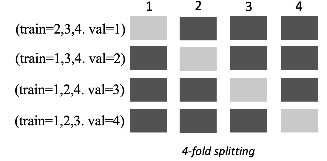
K-fold splitting

K-fold splitting is a method that separates an input training dataset into multiple training and validation datasets. The dataset is split into k equally-sized sub-samples called folds. Models are then trained on k-1 folds and tested against the remaining k^th fold, which is the validation dataset. The process is repeated k times using a different data set for validation.

The following image depicts k-fold splitting with k = 4 folds. Each fold is represented as a row. The dark-toned boxes represent the parts of the data used in training. The remaining light-toned boxes indicate the validation datasets.

Autopilot uses k-fold cross-validation for both hyperparameter optimization (HPO) mode and ensembling mode.

You can deploy Autopilot models that are built using cross-validation like you would with any other Autopilot or SageMaker model.

HPO mode

K-fold cross-validation uses the k-fold splitting method for cross-validation. In HPO mode, Autopilot automatically implements k-fold cross-validation for small datasets with 50,000 or fewer training instances. Performing cross-validation is especially important when training on small datasets because it protects against overfitting and selection bias.

HPO mode uses a k value of 5 on each of the candidate algorithms that are used to model the dataset. Multiple models are trained on different splits, and the models are stored separately. When training is complete, validation metrics for each of the models are averaged to produce a single estimation metric. Lastly, Autopilot combines the models from the trial with the best validation metric into an ensemble model. Autopilot uses this ensemble model to make predictions.

The validation metric for the models trained by Autopilot is presented as the objective metric in the model leaderboard. Autopilot uses the default validation metric for each problem type that it handles, unless you specify otherwise. For the list of all metrics that Autopilot uses, see Autopilot metrics.

For example, the Boston Housing dataset contains only 861 samples. If you build a model to predict house sale prices using this dataset without cross-validation, you risk training on a dataset that is not representative of the Boston housing stock. If you split the data only once into training and validation subsets, the training fold may only contain data mainly from the suburbs. As a result, you would train on data that isn't representative of the rest of the city. In this example, your model would likely overfit on this biased selection. K-fold cross-validation can reduce the risk of this kind of error by making full and randomized use of the available data for both training and validation.

Cross-validation can increase training times by an average of 20%. Training times may also increase significantly for complex datasets.

Note

In HPO mode, you can see the training and validation metrics from each fold in your /aws/sagemaker/TrainingJobs CloudWatch Logs. For more information about CloudWatch Logs, see Log Amazon SageMaker Events with Amazon CloudWatch.

Ensembling mode

Note

Autopilot supports sample weights in ensembling mode. For the list of available metrics supporting sample weights, see Autopilot metrics.

In ensembling mode, cross-validation is performed regardless of dataset size. Customers can either provide their own validation dataset and custom data split ratio, or let Autopilot split the dataset automatically into an 80-20% split ratio. The training data is then split into k-folds for cross-validation, where the value of k is determined by the AutoGluon engine. An ensemble consists of multiple machine learning models, where each model is known as the base model. A single base model is trained on (k-1) folds and makes out-of-fold predictions on the remaining fold. This process is repeated for all k folds, and the out-of-fold (OOF) predictions are concatenated to form a single set of predictions. All base models in the ensemble follow this same process of generating OOF predictions.

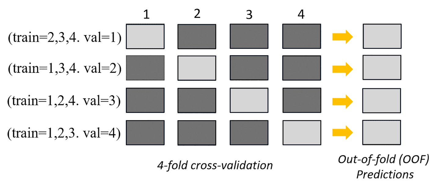
The following image depicts k-fold validation with k = 4 folds. Each fold is represented as a row. The dark-toned boxes represent the parts of the data used in training. The remaining light-toned boxes indicate the validation datasets.

In the upper part of the image, in each fold, the first base model makes predictions on the validation dataset after training on the training datasets. At each subsequent fold, the datasets change roles. A dataset that was previously used for training is now used for validation, and this also applies in reverse. At the end of k folds, all of the predictions are concatenated to form a single set of predictions called an out-of-fold (OOF) prediction. This process is repeated for each n base models.

The OOF predictions for each base model are then used as features to train a stacking model. The stacking model learns the importance weights for each base model. These weights are used to combine the OOF predictions to form the final prediction. Performance on the validation dataset determines which base or stacking model is the best, and this model is returned as the final model.

In ensemble mode, you can either provide your own validation dataset or let Autopilot split the input dataset automatically into 80% train and 20% validation datasets. The training data is then split into k-folds for cross-validation and produces an OOF prediction and a base model for each fold.

These OOF predictions are used as features to train a stacking model, which simultaneously learns weights for each base model. These weights are used to combine the OOF predictions to form the final prediction. The validation datasets for each fold are used for hyperparameter tuning of all base models and the stacking model. Performance on the validation datasets determines which base or stacking model is the best model, and this model is returned as the final model.