This whitepaper is for historical reference only. Some content might be outdated and some links might not be available.
Failure detection using outlier detection
One gap with the previous approach could arise when you see elevated error rates in multiple Availability Zones that are occurring for an uncorrelated reason. Imagine a scenario where you have EC2 instances deployed across three Availability Zones and your availability alarm threshold is 99%. Then, a single Availability Zone impairment occurs, isolating many instances and causes availability in that zone to drop to 55%. At the same time, but in a different Availability Zone, a single EC2 instance exhausts all of the storage on its EBS volume, and can no longer write logs files. This causes it to start returning errors, but it still passes the load balancer health checks because those don’t trigger a log file to be written. This results in availability dropping to 98% in that Availability Zone. In this case, your single Availability Zone impact alarm wouldn’t activate because you are seeing an availability impact in multiple Availability Zones. However, you could still mitigate almost all of the impact by evacuating the impaired Availability Zone.
In some types of workloads, you might experience errors consistently across all Availability Zones where the previous availability metric might not be useful. Take AWS Lambda for example. AWS allows customers to create their own code to run in the Lambda function. To use the service, you have to upload your code in a ZIP file, including dependencies, and define the entry point to the function. But sometimes customers get this part wrong, for example, they might forget a critical dependency in the ZIP file, or mistype the method name in the Lambda function definition. This causes the function to fail to be invoked and results in an error. AWS Lambda sees these kinds of errors all the time, but they’re not indicative that anything is necessarily unhealthy. However, something like an Availability Zone impairment might also cause these errors to appear.
To find signal in this kind of noise, you can use outlier detection to determine if there is a statistically significant skew in the number of errors among Availability Zones. Although we see errors across multiple Availability Zones, if there was truly a failure in one of them, we’d expect to see a much higher error rate in that Availability Zone compared to the other ones, or potentially much lower. But how much higher or lower?
One way to do this analysis is by using a chi-squared
A chi-squared test evaluates the probability that some distribution of results is likely to occur. In this case, we’re interested in the distribution of errors across some defined set of AZs. For this example, to make the math easier, consider four Availability Zones.
First, establish the null hypothesis, which defines what you believe the default outcome is. In this test, the null hypothesis is that you expect errors to be evenly distributed across each Availability Zone. Then, generate the alternative hypothesis, which is that the errors are not evenly distributed indicating an Availability Zone impairment. Now you can test these hypotheses using data from your metrics. For this purpose, you’ll sample your metrics from a five-minute window. Suppose you get 1000 published data points in that window, in which you see 100 total errors. You expect that with an even distribution the errors would occur 25% of the time in each of the four Availability Zones. Assume the following table shows what you expected compared to what you actually saw.
Table 1: Expected versus actual errors seen
| AZ | Expected | Actual |
|---|---|---|
use1-az1 |
25 | 20 |
use1-az2 |
25 | 20 |
use1-az3 |
25 | 25 |
use1-az4 |
25 | 35 |
So, you see that the distribution in reality isn’t even. However, you might believe that
this occurred due to some level of randomness in the data points you sampled. There’s some
level of probability that this type of distribution could occur in the sample set and still
assume that the null hypothesis is true. This leads to the following question: What is the
probability of getting a result at least this extreme? If that probability is below a defined
threshold, you reject the null hypothesis. To be statistically
significant
1 Craparo, Robert M. (2007). "Significance level". In Salkind, Neil J. Encyclopedia of Measurement and Statistics 3. Thousand Oaks, CA: SAGE Publications. pp. 889–891. ISBN 1-412-91611-9.
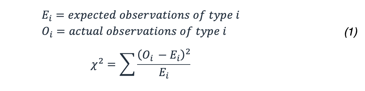
How do you calculate the probability of this outcome? You use the χ2 statistic that provides very well-studied distributions and can be used to determine the probability of getting a result this extreme or more extreme using this formula.
For our example, this results in:
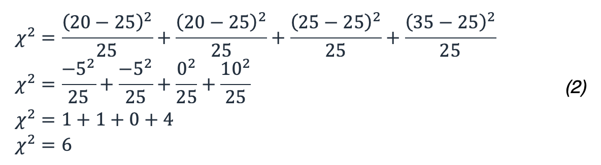
So, what does 6 mean in terms of our probability? You need to look at a
chi-squared distribution with the appropriate degree of freedom. The following figure shows
several chi-squared distributions for different degrees of freedom.
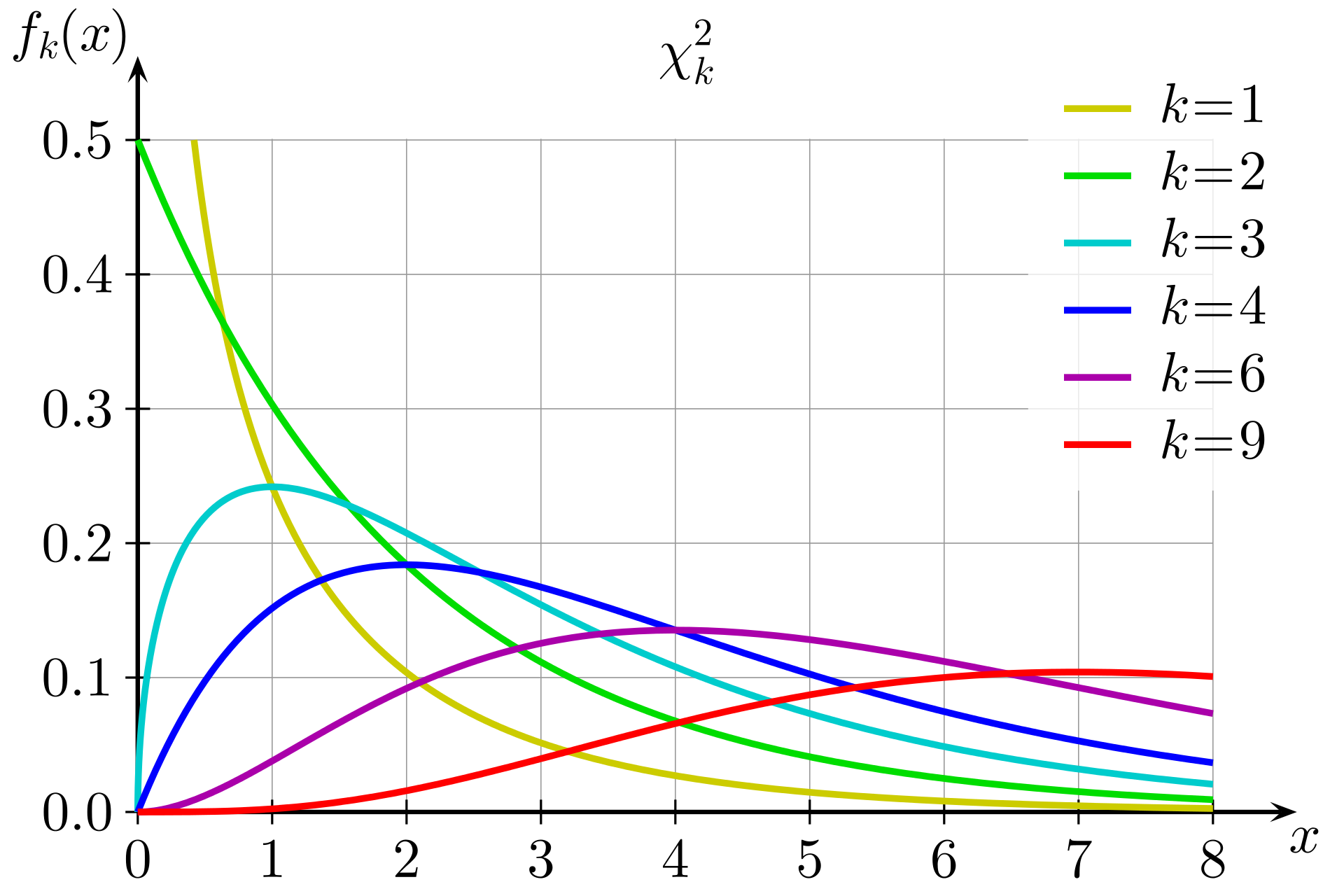
Chi-squared distributions for different degrees of freedom
The degree of freedom is calculated as one less than the number of choices in the test. In this case, because there are four Availability Zones, the degree of freedom is three. Then, you want to know the area under the curve (the integral) for x ≥ 6 on the k = 3 plot. You can also use a pre-calculated table with commonly used values to approximate that value.
Table 2: Chi-squared critical values
| Degrees of freedom | Probability less than the critical value | ||||
|---|---|---|---|---|---|
| 0.75 | 0.90 | 0.95 | 0.99 | 0.999 | |
| 1 | 1.323 | 2.706 | 3.841 | 6.635 | 10.828 |
| 2 | 2.773 | 4.605 | 5.991 | 9.210 | 13.816 |
| 3 | 4.108 | 6.251 | 7.815 | 11.345 | 16.266 |
| 4 | 5.385 | 7.779 | 9.488 | 13.277 | 18.467 |
For three degrees of freedom, the chi-squared value of six falls between the 0.75 and 0.9 probability columns. What this means is there is a greater than 10% chance of this distribution occurring, which is not less than the 5% threshold. Therefore, you accept the null hypothesis and determine there is not a statistically significant difference in error rates among the Availability Zones.
Performing a chi-squared statistics test isn’t natively supported in CloudWatch metric math, so you’ll need collect the applicable error metrics from CloudWatch and run the test in a compute environment like Lambda. You can decide to perform this test at something like an MVC Controller/Action or individual microservice level, or at the Availability Zone level. You’ll need to consider whether an Availability Zone impairment would affect each Controller/Action or microservice equally, or whether something like a DNS failure might cause impact in a low throughput service and not in a high throughput service, which could mask the impact when aggregated. In either case, select the appropriate dimensions to create the query. The level of granularity will also impact the resulting CloudWatch alarms you create.
Collect the error count metric for each AZ and Controller/Action in a specified time window. First, calculate the result of the chi-squared test as either true (there was a statistically significant skew) or false (there was wasn’t, that is, the null hypothesis holds). If the result is false, publish a 0 data point to your metric stream for chi-squared results for each Availability Zone. If the result is true, publish a 1 data point for the Availability Zone with the errors farthest from the expected value and a 0 for the others (refer to Appendix B – Example chi-squared calculation for sample code that can be used in a Lambda function). You can follow the same approach as the previous availability alarms by using creating a 3 in a row CloudWatch metric alarm and a 3 out of 5 CloudWatch metric alarm based on the data points being produced by the Lambda function. As in the previous examples, this approach can be modified to use more or less data points in a shorter or longer window.
Then, add these alarms to your existing Availability Zone availability alarm for the Controller and Action combination, shown in the following figure.
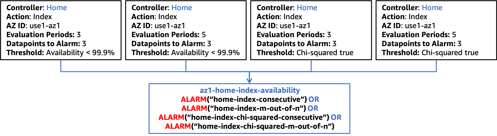
Integrating the chi-squared statistics test with composite alarms
As mentioned previously, when you onboard new functionality in your workload, you only need to create the appropriate CloudWatch metric alarms that are specific to that new functionality and update the next tier in the composite alarm hierarchy to include those alarms. The rest of the alarm structure remains static.
