Use the SageMaker AI DeepAR forecasting algorithm
The Amazon SageMaker AI DeepAR forecasting algorithm is a supervised learning algorithm for forecasting scalar (one-dimensional) time series using recurrent neural networks (RNN). Classical forecasting methods, such as autoregressive integrated moving average (ARIMA) or exponential smoothing (ETS), fit a single model to each individual time series. They then use that model to extrapolate the time series into the future.
In many applications, however, you have many similar time series across a set of cross-sectional units. For example, you might have time series groupings for demand for different products, server loads, and requests for webpages. For this type of application, you can benefit from training a single model jointly over all of the time series. DeepAR takes this approach. When your dataset contains hundreds of related time series, DeepAR outperforms the standard ARIMA and ETS methods. You can also use the trained model to generate forecasts for new time series that are similar to the ones it has been trained on.
The training input for the DeepAR algorithm is one or, preferably, more
target time series that have been generated by the same process or similar
processes. Based on this input dataset, the algorithm trains a model that learns an
approximation of this process/processes and uses it to predict how the target time series
evolves. Each target time series can be optionally associated with a vector of static
(time-independent) categorical features provided by the cat field and a vector
of dynamic (time-dependent) time series provided by the dynamic_feat field.
SageMaker AI trains the DeepAR model by randomly sampling training examples from each target time
series in the training dataset. Each training example consists of a pair of adjacent context
and prediction windows with fixed predefined lengths. To control how far in the past the
network can see, use the context_length hyperparameter. To control how far in
the future predictions can be made, use the prediction_length hyperparameter.
For more information, see How the DeepAR Algorithm Works.
Topics
Input/Output Interface for the DeepAR Algorithm
DeepAR supports two data channels. The required train channel describes
the training dataset. The optional test channel describes a dataset that
the algorithm uses to evaluate model accuracy after training. You can provide training
and test datasets in JSON Lines
When specifying the paths for the training and test data, you can specify a single file or a directory that contains multiple files, which can be stored in subdirectories. If you specify a directory, DeepAR uses all files in the directory as inputs for the corresponding channel, except those that start with a period (.) and those named _SUCCESS. This ensures that you can directly use output folders produced by Spark jobs as input channels for your DeepAR training jobs.
By default, the DeepAR model determines the input format from the file extension
(.json, .json.gz, or .parquet) in the
specified input path. If the path does not end in one of these extensions, you must
explicitly specify the format in the SDK for Python. Use the content_type
parameter of the InputData
The records in your input files should contain the following fields:
-
start—A string with the formatYYYY-MM-DD HH:MM:SS. The start timestamp can't contain time zone information. -
target—An array of floating-point values or integers that represent the time series. You can encode missing values asnullliterals, or as"NaN"strings in JSON, or asnanfloating-point values in Parquet. -
dynamic_feat(optional)—An array of arrays of floating-point values or integers that represents the vector of custom feature time series (dynamic features). If you set this field, all records must have the same number of inner arrays (the same number of feature time series). In addition, each inner array must be the same length as the associatedtargetvalue plusprediction_length. Missing values are not supported in the features. For example, if target time series represents the demand of different products, an associateddynamic_featmight be a boolean time-series which indicates whether a promotion was applied (1) to the particular product or not (0):{"start": ..., "target": [1, 5, 10, 2], "dynamic_feat": [[0, 1, 1, 0]]} -
cat(optional)—An array of categorical features that can be used to encode the groups that the record belongs to. Categorical features must be encoded as a 0-based sequence of positive integers. For example, the categorical domain {R, G, B} can be encoded as {0, 1, 2}. All values from each categorical domain must be represented in the training dataset. That's because the DeepAR algorithm can forecast only for categories that have been observed during training. And, each categorical feature is embedded in a low-dimensional space whose dimensionality is controlled by theembedding_dimensionhyperparameter. For more information, see DeepAR Hyperparameters.
If you use a JSON file, it must be in JSON
Lines
{"start": "2009-11-01 00:00:00", "target": [4.3, "NaN", 5.1, ...], "cat": [0, 1], "dynamic_feat": [[1.1, 1.2, 0.5, ...]]}
{"start": "2012-01-30 00:00:00", "target": [1.0, -5.0, ...], "cat": [2, 3], "dynamic_feat": [[1.1, 2.05, ...]]}
{"start": "1999-01-30 00:00:00", "target": [2.0, 1.0], "cat": [1, 4], "dynamic_feat": [[1.3, 0.4]]}
In this example, each time series has two associated categorical features and one time series features.
For Parquet, you use the
same
three fields as
columns.
In addition, "start" can be the datetime type. You can
compress Parquet files using gzip (gzip) or the Snappy compression library
(snappy).
If the algorithm is trained without cat and dynamic_feat
fields, it learns a "global" model, that is a model that is agnostic to the specific
identity of the target time series at inference time and is conditioned only on its
shape.
If the model is conditioned on the cat and dynamic_feat
feature data provided for each time series, the prediction will probably be influenced
by the character of time series with the corresponding cat features. For
example, if the target time series represents the demand of clothing items,
you can associate a two-dimensional cat vector that encodes the type of
item (e.g. 0 = shoes, 1 = dress) in the first component and the color of an item (e.g. 0
= red, 1 = blue) in the second component. A sample input would look as follows:
{ "start": ..., "target": ..., "cat": [0, 0], ... } # red shoes
{ "start": ..., "target": ..., "cat": [1, 1], ... } # blue dress
At inference time, you can request predictions for targets with cat
values that are combinations of the cat values observed in the training
data, for example:
{ "start": ..., "target": ..., "cat": [0, 1], ... } # blue shoes
{ "start": ..., "target": ..., "cat": [1, 0], ... } # red dress
The following guidelines apply to training data:
-
The start time and length of the time series can differ. For example, in marketing, products often enter a retail catalog at different dates, so their start dates naturally differ. But all series must have the same frequency, number of categorical features, and number of dynamic features.
-
Shuffle the training file with respect to the position of the time series in the file. In other words, the time series should occur in random order in the file.
-
Make sure to set the
startfield correctly. The algorithm uses thestarttimestamp to derive the internal features. -
If you use categorical features (
cat), all time series must have the same number of categorical features. If the dataset contains thecatfield, the algorithm uses it and extracts the cardinality of the groups from the dataset. By default,cardinalityis"auto". If the dataset contains thecatfield, but you don't want to use it, you can disable it by settingcardinalityto"". If a model was trained using acatfeature, you must include it for inference. -
If your dataset contains the
dynamic_featfield, the algorithm uses it automatically. All time series have to have the same number of feature time series. The time points in each of the feature time series correspond one-to-one to the time points in the target. In addition, the entry in thedynamic_featfield should have the same length as thetarget. If the dataset contains thedynamic_featfield, but you don't want to use it, disable it by setting(num_dynamic_featto""). If the model was trained with thedynamic_featfield, you must provide this field for inference. In addition, each of the features has to have the length of the provided target plus theprediction_length. In other words, you must provide the feature value in the future.
If you specify optional test channel data, the DeepAR algorithm evaluates the trained model with different accuracy metrics. The algorithm calculates the root mean square error (RMSE) over the test data as follows:
-y(i,t))^2)).](/images/sagemaker/latest/dg/images/deepar-1.png)
yi,t
is the true value of time series i at the time
t.
ŷi,t
is the mean prediction. The sum is over all n time series in the
test set and over the last Τ time points for each time series, where Τ
corresponds to the forecast horizon. You specify the length of the forecast horizon by
setting the prediction_length hyperparameter. For more information, see
DeepAR Hyperparameters.
In addition, the algorithm evaluates the accuracy of the forecast distribution using weighted quantile loss. For a quantile in the range [0, 1], the weighted quantile loss is defined as follows:
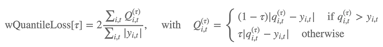
qi,t(τ)
is the τ-quantile of the distribution that the model predicts. To specify which
quantiles to calculate loss for, set the test_quantiles hyperparameter. In
addition to these, the average of the prescribed quantile losses is reported as part of
the training logs. For information, see DeepAR Hyperparameters.
For inference, DeepAR accepts JSON format and the following fields:
-
"instances", which includes one or more time series in JSON Lines format -
A name of
"configuration", which includes parameters for generating the forecast
For more information, see DeepAR Inference Formats.
Best Practices for Using the DeepAR Algorithm
When preparing your time series data, follow these best practices to achieve the best results:
-
Except for when splitting your dataset for training and testing, always provide the entire time series for training, testing, and when calling the model for inference. Regardless of how you set
context_length, don't break up the time series or provide only a part of it. The model uses data points further back than the value set incontext_lengthfor the lagged values feature. -
When tuning a DeepAR model, you can split the dataset to create a training dataset and a test dataset. In a typical evaluation, you would test the model on the same time series used for training, but on the future
prediction_lengthtime points that follow immediately after the last time point visible during training. You can create training and test datasets that satisfy this criteria by using the entire dataset (the full length of all time series that are available) as a test set and removing the lastprediction_lengthpoints from each time series for training. During training, the model doesn't see the target values for time points on which it is evaluated during testing. During testing, the algorithm withholds the lastprediction_lengthpoints of each time series in the test set and generates a prediction. Then it compares the forecast with the withheld values. You can create more complex evaluations by repeating time series multiple times in the test set, but cutting them at different endpoints. With this approach, accuracy metrics are averaged over multiple forecasts from different time points. For more information, see Tune a DeepAR Model. -
Avoid using very large values (>400) for the
prediction_lengthbecause it makes the model slow and less accurate. If you want to forecast further into the future, consider aggregating your data at a lower frequency. For example, use5mininstead of1min. -
Because lags are used, a model can look further back in the time series than the value specified for
context_length. Therefore, you don't need to set this parameter to a large value. We recommend starting with the value that you used forprediction_length. -
We recommend training a DeepAR model on as many time series as are available. Although a DeepAR model trained on a single time series might work well, standard forecasting algorithms, such as ARIMA or ETS, might provide more accurate results. The DeepAR algorithm starts to outperform the standard methods when your dataset contains hundreds of related time series. Currently, DeepAR requires that the total number of observations available across all training time series is at least 300.
EC2 Instance Recommendations for the DeepAR Algorithm
You can train DeepAR on both GPU and CPU instances and in both single and multi-machine settings. We recommend starting with a single CPU instance (for example, ml.c4.2xlarge or ml.c4.4xlarge), and switching to GPU instances and multiple machines only when necessary. Using GPUs and multiple machines improves throughput only for larger models (with many cells per layer and many layers) and for large mini-batch sizes (for example, greater than 512).
For inference, DeepAR supports only CPU instances.
Specifying large values for context_length,
prediction_length, num_cells, num_layers, or
mini_batch_size can create models that are too large for small
instances. In this case, use a larger instance type or reduce the values for these
parameters. This problem also frequently occurs when running hyperparameter tuning jobs.
In that case, use an instance type large enough for the model tuning job and consider
limiting the upper values of the critical parameters to avoid job failures.
DeepAR Sample Notebooks
For a sample notebook that shows how to prepare a time series dataset for training the
SageMaker AI DeepAR algorithm and how to deploy the trained model for performing inferences, see
DeepAR demo on electricity dataset
For more information about the Amazon SageMaker AI DeepAR algorithm, see the following blog posts:
