Introduction to Model Parallelism

Model parallelism is a distributed training method in which the deep learning model is partitioned across multiple devices, within or across instances. This introduction page provides a high-level overview about model parallelism, a description of how it can help overcome issues that arise when training DL models that are typically very large in size, and examples of what the SageMaker model parallel library offers to help manage model parallel strategies as well as memory consumption.

What is Model Parallelism?

Increasing the size of deep learning models (layers and parameters) yields better accuracy for complex tasks such as computer vision and natural language processing. However, there is a limit to the maximum model size you can fit in the memory of a single GPU. When training DL models, GPU memory limitations can be bottlenecks in the following ways:

• They limit the size of the model you can train, since the memory footprint of a model scales proportionally to the number of parameters.

• They limit the per-GPU batch size during training, driving down GPU utilization and training efficiency.

To overcome the limitations associated with training a model on a single GPU, SageMaker provides the model parallel library to help distribute and train DL models efficiently on multiple compute nodes. Furthermore, with the library, you can achieve most optimized distributed training using EFA-supported devices, which enhance the performance of inter-node communication with low latency, high throughput, and OS bypass.

Estimate Memory Requirements Before Using Model Parallelism

Before you use the SageMaker model parallel library, consider the following to get a sense of the memory requirements of training large DL models.

For a training job that uses AMP (FP16) and Adam optimizers, the required GPU memory per parameter is about 20 bytes, which we can break down as follows:

• An FP16 parameter ~ 2 bytes

• An FP16 gradient ~ 2 bytes

• An FP32 optimizer state ~ 8 bytes based on the Adam optimizers

• An FP32 copy of parameter ~ 4 bytes (needed for the optimizer apply (OA) operation)

• An FP32 copy of gradient ~ 4 bytes (needed for the OA operation)

Even for a relatively small DL model with 10 billion parameters, it can require at least 200GB of memory, which is much larger than the typical GPU memory (for example, NVIDIA A100 with 40GB/80GB memory and V100 with 16/32 GB) available on a single GPU. Note that on top of the memory requirements for model and optimizer states, there are other memory consumers such as activations generated in the forward pass. The memory required can be a lot greater than 200GB.

For distributed training, we recommend that you use Amazon EC2 P3 and P4 instances that have NVIDIA V100 and A100 Tensor Core GPUs respectively. For more details about specifications such as CPU cores, RAM, attached storage volume, and network bandwidth, see the Accelerated Computing section in the Amazon EC2 Instance Types page.

Even with the accelerated computing instances, it is obvious that models with about 10 billion parameters such as Megatron-LM and T5 and even larger models with hundreds of billions of parameters such as GPT-3 cannot fit model replicas in each GPU device.

How the Library Employs Model Parallelism and Memory Saving Techniques

The library consists of various types of model parallelism features and memory-saving features such as optimizer state sharding, activation checkpointing, and activation offloading. All these techniques can be combined to efficiently train large models that consist of hundreds of billions of parameters.

Sharded data parallelism (available for PyTorch)

Sharded data parallelism is a memory-saving distributed training technique that splits the state of a model (model parameters, gradients, and optimizer states) across GPUs within a data-parallel group.

SageMaker implements sharded data parallelism through the implementation of MiCS, which is a library that minimizes communication scale and discussed in the blog post Near-linear scaling of gigantic-model training on AWS.

You can apply sharded data parallelism to your model as a stand-alone strategy. Furthermore, if you are using the most performant GPU instances equipped with NVIDIA A100 Tensor Core GPUs, ml.p4d.24xlarge, you can take the advantage of improved training speed from the AllGather operation offered by SMDDP Collectives.

To dive deep into sharded data parallelism and learn how to set it up or use a combination of sharded data parallelism with other techniques like tensor parallelism and FP16 training, see Sharded Data Parallelism.

Pipeline parallelism (available for PyTorch and TensorFlow)

Pipeline parallelism partitions the set of layers or operations across the set of devices, leaving each operation intact. When you specify a value for the number of model partitions (pipeline_parallel_degree), the total number of GPUs (processes_per_host) must be divisible by the number of the model partitions. To set this up properly, you have to specify the correct values for the pipeline_parallel_degree and processes_per_host parameters. The simple math is as follows:

(pipeline_parallel_degree) x (data_parallel_degree) = processes_per_host

The library takes care of calculating the number of model replicas (also called data_parallel_degree) given the two input parameters you provide.

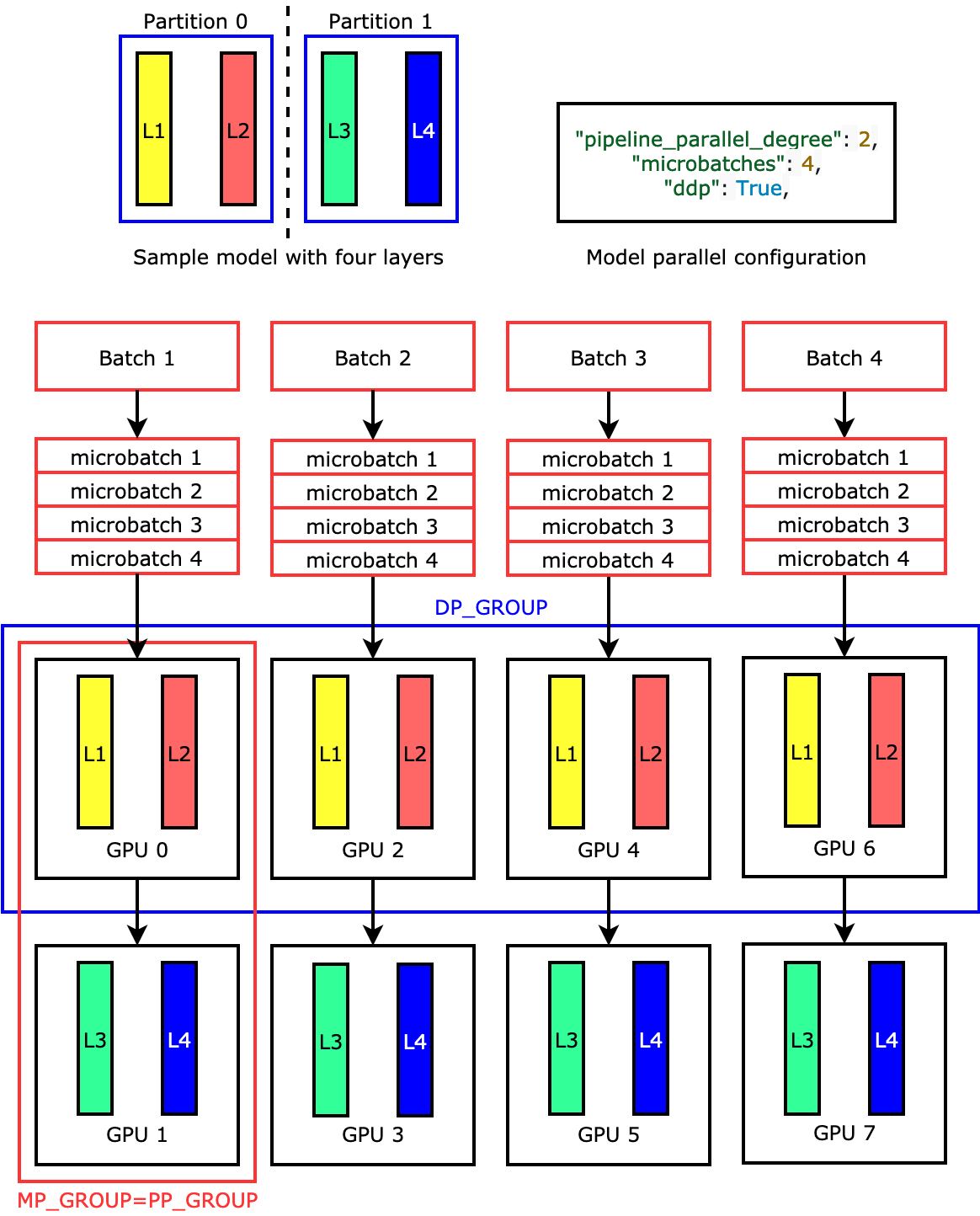
For example, if you set "pipeline_parallel_degree": 2 and "processes_per_host": 8 to use an ML instance with eight GPU workers such as ml.p3.16xlarge, the library automatically sets up the distributed model across the GPUs and four-way data parallelism. The following image illustrates how a model is distributed across the eight GPUs achieving four-way data parallelism and two-way pipeline parallelism. Each model replica, where we define it as a pipeline parallel group and label it as PP_GROUP, is partitioned across two GPUs. Each partition of the model is assigned to four GPUs, where the four partition replicas are in a data parallel group and labeled as DP_GROUP. Without tensor parallelism, the pipeline parallel group is essentially the model parallel group.

To dive deep into pipeline parallelism, see Core Features of the SageMaker Model Parallelism Library.

To get started with running your model using pipeline parallelism, see Run a SageMaker Distributed Training Job with the SageMaker Model Parallel Library.

Tensor parallelism (available for PyTorch)

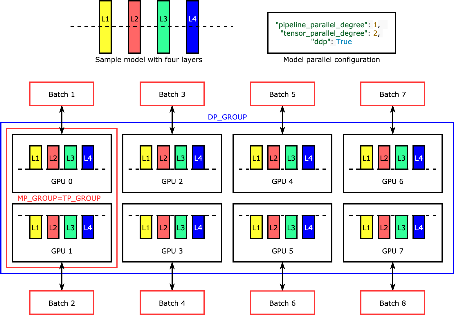
Tensor parallelism splits individual layers, or nn.Modules, across devices, to be run in parallel. The following figure shows the simplest example of how the library splits a model with four layers to achieve two-way tensor parallelism ("tensor_parallel_degree": 2). The layers of each model replica are bisected and distributed into two GPUs. In this example case, the model parallel configuration also includes "pipeline_parallel_degree": 1 and "ddp": True (uses PyTorch DistributedDataParallel package in the background), so the degree of data parallelism becomes eight. The library manages communication across the tensor-distributed model replicas.

The usefulness of this feature is in the fact that you can select specific layers or a subset of layers to apply tensor parallelism. To dive deep into tensor parallelism and other memory-saving features for PyTorch, and to learn how to set a combination of pipeline and tensor parallelism, see Tensor Parallelism.

Optimizer state sharding (available for PyTorch)

To understand how the library performs optimizer state sharding, consider a simple example model with four layers. The key idea in optimizing state sharding is you don't need to replicate your optimizer state in all of your GPUs. Instead, a single replica of the optimizer state is sharded across data-parallel ranks, with no redundancy across devices. For example, GPU 0 holds the optimizer state for layer one, the next GPU 1 holds the optimizer state for L2, and so on. The following animated figure shows a backward propagation with the optimizer state sharding technique. At the end of the backward propagation, there's compute and network time for the optimizer apply (OA) operation to update optimizer states and the all-gather (AG) operation to update the model parameters for the next iteration. Most importantly, the reduce operation can overlap with the compute on GPU 0, resulting in a more memory-efficient and faster backward propagation. In the current implementation, AG and OA operations do not overlap with compute. It can result in an extended computation during the AG operation, so there might be a tradeoff.

For more information about how to use this feature, see Optimizer State Sharding.

Activation offloading and checkpointing (available for PyTorch)

To save GPU memory, the library supports activation checkpointing to avoid storing internal activations in the GPU memory for user-specified modules during the forward pass. The library recomputes these activations during the backward pass. In addition, the activation offloading feature offloads the stored activations to CPU memory and fetches back to GPU during the backward pass to further reduce activation memory footprint. For more information about how to use these features, see Activation Checkpointing and Activation Offloading.

Choosing the right techniques for your model

For more information about choosing the right techniques and configurations, see SageMaker Distributed Model Parallel Best Practices and Configuration Tips and Pitfalls.