Addressing the challenges with demand forecasting solutions on AWS

This section dives deeper into the previously mentioned challenges, and provides solutions.

Adequate data to start: sources of data and data handling

In a well-architected solution, the data follows through a well-defined pattern of creation, ingestion, storage, and consumption layers where the consumption bears the forecasting stage. Whether the data is consumed by business partners or by data scientists, you may want to centralize the data to get more insights. In some cases, the data is created at the edge or by third parties. In these cases, customers can subscribe to new data to enhance their existing data. We provide third-party subscriptions to utilize the data without any hassle, including billing and data source management solutions.

Typically, the data required for demand forecasting is in the form of time series and metadata. You can use Amazon Simple Storage Service (Amazon S3) to store time series data and metadata typically in CSV format. You can directly use this data to employ Amazon SageMaker AI solutions which will be explained in the following section. If you are using Amazon Forecast for the demand forecasting, you can upload your time series and metadata data to Amazon Forecast. Follow the instructions in Prepare and clean your data for Amazon Forecast to prepare and upload your data to Amazon Forecast.

Solutions

Data is created at the edge, on your ecommerce site, or from social media by customers. You can use external connectors to direct data to your data storage on AWS. Use the AWS Marketplace to find other readily available connectors. This solution can be unified as a data lake on AWS, where you can not only use ML inference for demand forecasting, you can also perform data lifecycle management and analytics. If you have data on-premises, you can keep your data on-premises if you want, and add a connection to your data through AWS Storage Gateway. You can use data lakes on AWS to build a flexible and hybrid architecture.

External data ingestion

The other specific application for industrial, in-demand forecasting is the Internet of Things (IoT). Some of our customers have IoT devices on their production or manufacturing sites, with sensors or telemetry data coming from the devices. These customers may want to use their IoT data in their demand forecasting. You can utilize AWS IoT Analytics solutions to incorporate an IoT workload into the solutions provided in this document.

Customers may also look for external data resources to gather a wide-variety of data to forecast. These resources can include industry trends, society information, social media posts, and so on. You can subscribe to AWS Data Exchange to get third-party data to enhance your models. The advantage of this method is the ease of data utilization with APIs. Payment is easy, because your subscription billing will be paid to the third party as part of your AWS Billing and Cost Management.

Data science expertise: empower your development teams with Amazon ML services

In this section, we address the data science expertise pain point, and the solutions for teams with and without data science expertise and pinpoint the services to cover a wide-variety of organizations.

Teams with data science expertise

Amazon SageMaker AI can empower customers with or without dedicated data science teams or developers. However, it is the recommended service for teams with data-science expertise. Amazon SageMaker AI brings agility, innovation, and automation to existing data science teams. SageMaker AI acts as the single source of all data-science related projects covering complete ML application lifecycle from data ingestion to model monitoring and lifecycle management. Amazon SageMaker AI comes with a fully-developed, user-friendly Integrated Development Environment (IDE) called SageMaker AI Studio. You can start reinventing your business by empowering your data-science teams with Amazon SageMaker AI through Studio IDE.

The following figure summarizes a common pattern of Amazon SageMaker AI experience for data scientists or developers who perform demand forecasting. It starts with training data located in an S3 bucket (step 1). Amazon SageMaker AI utilizes Jupyter Notebook (step 2). Here, you can use Amazon SageMaker AI SDK for Python. R practitioners can also use SageMaker AI. Later, the model is trained (step 3) and the endpoint is deployed (step 4). Here you can monitor and log your SageMaker AI deployment and endpoint using Amazon CloudWatch (step 5) and finally using input data for inference located in S3, the prediction requests can be sent to the SageMaker AI endpoint and make predictions (step 6).

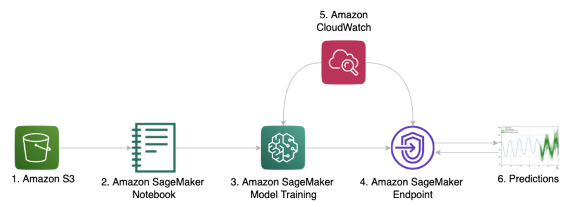
A common pattern of using Amazon SageMaker AI – training data in Amazon S3 and an inference endpoint deployed for production.

Starting with a well-documented, organized, and well-architected solution can be the fastest and the productive step to take. Some data scientists may want to start with Amazon SageMaker AI deployment without an empty-page, meaning they may want to utilize a readily available, best practiced, and fully developed solution to start with.

Amazon SageMaker AI JumpStart provides developers and data science teams ready-to-start AI/ML models and pipelines. SageMaker AI JumpStart can be used as-is, because it is ready to be deployed. Also, you can consider incrementally training your data or modifying the code based on your needs.

For demand forecasting, SageMaker AI JumpStart comes with a pre-trained, deep learning-based forecasting model, using Long- and Short-Term Temporal Patterns with Deep Neural Network (LSTNet). LSTNet is a state-of-the-art multi-variate (made of multiple correlated time series data) forecasting model, as explained in Cornell University’s paper, Modeling Long- and Short-Term Temporal Patterns with Deep Neural Networks.

Deep learning-based demand forecasting with LSTNet uses the short-term and long-term effects of the historical data, which may not be accurately captured by conventional time series analyses such as autoregressive integrated moving average (ARIMA) or exponential smoothing (ETS) methods. This is especially important in forecasting complex behaviors in real-life businesses such as energy industry or retail.

To start using the deep learning model (LSTNet-based) with JumpStart, refer to this documentation. The output of the model is a trained model which can be deployed on your inference selection. Recently, Amazon SageMaker AI has added serverless inference to have a cost model of per inference for unpredictable traffics. Alternatively, you can use Amazon SageMaker AI Inference Recommender to get a data-based recommendation for your endpoint.

Amazon SageMaker AI comes with state-of-the-art time series algorithms using deep learning. Along with LSTNet, SageMaker AI provides DeepAR. Similar to LSTNet, DeepAR is a supervised learning algorithm for forecasting one-dimensional time series recurrent neural networks (RNN). Generally, demand forecasting in CPG, manufacturing, and energy industries comes with hundreds of similar time series across a set of business metrics.

Note

Deep learning models require a large amount of data, whereas conventional approaches such as ARIMA can start with data less than 100 data points.

For example, you may have demand data for wide variety of products, webpages, or households’ electricity and gas usage. For this type of application, you can benefit from training a single model jointly over all of the time series to a one-dimensional output, which is demand. DeepAR takes this approach. Another deep learning model for demand forecasting is Prophet due to its excellence in considering seasonality effects. Refer to Deep demand forecasting with Amazon SageMaker AI, which compares the performance, cost, and accuracy of these models in demand-forecasting. The decision for the best model may not mean the highest accuracy for all users.

For some, an adequate accuracy with lower latency and faster training is a better option than a high accuracy but more expensive model. To bring automation and innovation, your data science or ML teams may want to experiment with other models to see which model works the best. For more information, refer to the Amazon SageMaker AI Experiments – Organize, Track And Compare Your Machine Learning Trainings blog post.

Data scientists may want to perform advanced data preparation for their time series data built for ML purposes using Amazon SageMaker AI Data Wrangler, as explained in the Prepare time series data with Amazon SageMaker AI Data Wrangler blog post. Data Wrangler enables your data scientist to quickly analyze, visualize, transform, and clean data with ease.

For a constantly changing business environment, such as in the retail sector, the model can easily drift to show lower accuracy in time. Use SageMaker AI Model Monitor and then an auto-training with an MLOps through Amazon SageMaker AI Pipelines to speed up your model deployments and create a full pipeline to integrate CI/CD pipelines to your model development and deployments.

Teams without data science expertise

Use of SageMaker AI is possible for teams without data science expertise by using Amazon SageMaker AI Canvas. With Canvas, you can start utilizing predictive analyses for demand forecasting without any coding skills. Refer to Reinventing retail with no-code machine learning: Sales forecasting using Amazon SageMaker AI Canvas.

SageMaker AI Canvas brings drag-and-drop style user-friendly user-interface. Canvas gives a complete lifecycle of AI/ML deployment: connect, access, join data, and create datasets for model training with automatic data cleansing and model monitoring. Canvas can automatically engage ML models for your use case, which still allows you to configure your model based on your use case.

Your developers can share the model and dataset with other teams (such as a data science team in future or a business intelligence team) to review and provide feedback. For customers who want to start AI/ML without any expertise, Canvas is a good option to consider. In this case, you don’t have SageMaker AI, but rather a fully-managed service where you do not worry about provisioning, managing, administrating, or any related activity to start using AI/ML technologies.

Amazon Forecast

For demand forecasting, you can use Amazon Forecast. Amazon Forecast can fully enable businesses, such as utilities and manufacturing, with modern forecasting vision by providing high quality forecasting using state-of-the-art forecasting algorithms. Amazon Forecast comes with six algorithms; ARIMA, CNN-QR, DeepAR+, ETS, Non-Parametric Time Series (NPTS), and Prophet.

Amazon Forecast puts the power of Amazon’s extensive forecasting experience into the hands of all developers, without requiring ML expertise. Amazon Forecast comes with an AutoML option (refer to Training Predictors in the Amazon Forecast Developer Guide), including common patterns such as holidays, weather, and many more features perfecting a forecast. It is a fully managed service that delivers highly accurate forecasts, up to 50% more accurate than traditional methods.

As shown in the following figure, you can input your historical demand data in Amazon Forecast (only target data or some optional related data). The service then automatically sets up a data pipeline, ingests the input data, and trains a model (out of many algorithms, it can automatically choose the best performing model). Forecast then generates forecasts. It also identifies features that apply the most to the algorithm, and automatically tunes hyperparameters. Forecast then hosts your models so you can easily query them when needed. In the background, Forecast automatically cleans up resources you no longer use.

Time series forecasting with Amazon Forecast

With all of this work done behind the scene, you can save by not building your own ML expert team or resources to maintain your own in-house models.

In summary, Amazon Forecast is designed with these three main benefits in minds:

• Accuracy — Amazon Forecast uses deep neural networks and traditional statistical methods for forecasting. It can learn from historical data automatically, and pick the best algorithms to train a model designed for the data. When there are many related time series forecasts models (such as historical sales data of different items or historical electric load of different circuits) generated using the Amazon Forecast deep learning algorithms provides more accurate and efficient forecasts.

• End-to-end management — With Amazon Forecast, the entire forecasting workflow, from data upload to data processing, model training, dataset updates, and forecasting, can be automated. Then business planning tools or systems can directly consume Amazon forecasts as an API.

• Usability — With Amazon Forecast, you can look up and visualize forecasts for any time series at different granularities. Developers with no ML expertise can use the APIs, AWS Command Line Interface (AWS CLI), or the AWS Management Console to import training data into one or more Amazon Forecast datasets, train models, and deploy the models to generate forecasts.

Following are two case studies for customers who used Amazon Forecast for their demand forecasting.

Case study 1— Foxconn

Foxconn built an end-to-end demand forecasting solution in two months with Amazon Forecast. Foxconn manufactures some of the most widely used electronics worldwide such as laptops, phones. Customers are large electronics brands like Dell, HP, Lenovo, Apple.

Assembling these products is a highly manual process. Foxconn’s primary use case was to manage staffing by better estimating demand and production needs. Overstaffing means unused worker hours, while understaffing means overtime pay. Overtime pay is less costly.

Two main questions needed to answer were:

1. How many workers to call into the factory to meet short-term production needs for1 week ahead?

2. How many workers need to hire in the future in order to meet long-term production needs for 13 weeks ahead?

Foxconn had just over a dozen SKUs with 3+ years of daily historical demand data. Previous forecasting approach was to use forecast provided by Foxconn’s customers. With COVID-19 these forecasts became less reliable and labor costs increased as a result.

Foxconn decided to use Amazon Forecast for their demand forecasting. The whole process (importing data, model training and evaluation) took 6 weeks from start to finish. Initial solution provided 8% forecast accuracy improvement and an estimated $553K in annual savings.

Case study 2 — More Retail Ltd. (MRL)

More Retail Ltd. (MRL) is one of India’s top four grocery retailers, with a revenue in the order of several billion dollars. It has a store network of 22 hypermarkets and 624 supermarkets across India, supported by a supply chain of 13 distribution centers, 7 fruits and vegetables collection centers, and 6 staples processing centers.

Forecasting demand for the fresh produce category is challenging because fresh products have a short shelf life. With over-forecasting, stores end up selling stale or over-ripe products, or throw away most of their inventory (termed as shrinkage). If under-forecasted, products may be out of stock, which affects customer experience.

Customers may abandon their cart if they can’t find key items in their shopping list, because they don’t want to wait in checkout lines for just a handful of products. To add to this complexity, MRL has many SKUs across its over 600 supermarkets, leading to more than 6,000 store-SKU combinations.

With such a large network, it’s critical for MRL to deliver the right product quality at the right economic value, while meeting customer demand and keeping operational costs to a minimum. MRL collaborated with Ganit as its AI analytics partner to forecast demand with greater accuracy and build an automated ordering system to overcome the bottlenecks and deficiencies of manual judgment by store managers.

MRL used Amazon Forecast to increase their forecasting accuracy from 24% to 76%, leading to a reduction in wastage by up to 30% in the fresh produce category, improving in-stock rates from 80% to 90%, and increasing gross profit by 25%.

Building competitive demand forecasting models

The spectrum of model complexity changes from simple auto-regression extrapolation (such as ARIMA) to deep learning (such as DeepAR) models. In today’s complex and competitive business environment, most customers go with state-of-the-art deep learning models, as presented in the previous chapter.

Even if you decide to start with a deep learning model, the heavy lifting of training your selected model and optimizing model hyperparameters remain a challenge. The Amazon SageMaker AI training technologies help you to achieve your goals.

SageMaker AI hyperparameter tuning can also perform the optimization of finding the best hyperparameters based on your objective. During the process, SageMaker AI Debugger can debug, monitor, and profile training jobs in near real-time, detect conditions, optimize resource utilization by reducing bottlenecks, improve training time, and reduce costs of machine learning models.

You can still use traditional time series analyses such as auto-regression models on SageMaker AI. Due to the simplicity of those models, you can use traditional methods to code the model and run analysis on SageMaker AI notebooks. You can also create your own models from scratch on SageMaker AI and keep them as container images to perform model/instance lifecycles as if they are SageMaker AI models, so you can use all of the applicable SageMaker AI features.

You can develop your own advanced demand forecasting ML solutions. For example, one of the advanced applications is to employ hierarchical time series forecasting using Amazon SageMaker AI. This approach considers the hierarchical relationship between the data groups, of which overall combined effects form the demand (for example, a store is in a city, a city is in a state, and so on). Once your model is developed by your data scientists or engineers, you can package models in a container and start using the container image as a reference.

Here you can use model versioning, using SageMaker AI Model Registry so your engineers work on these reusable assets (models in containers) just like they can with built-in SageMaker AI models. Refer to Building your own algorithm container.

The other option is to use Amazon Forecast and SageMaker AI Canvas to completely overhaul the optimization, giving the heavy lifting to AWS. Amazon Forecast has many time series models, including autoregressive and advanced models, so you can start performing demand forecasting through the Amazon Forecast APIs. SageMaker AI Canvas gives you a short-no-code distance to SageMaker AI capabilities.

Model lifecycle and ML operations (MLOps) for robust demand forecasting

Any forecasting model will drift over time, creating inaccurate predictions. Along with drift, new models and technologies emerge, requiring a model lifecycle. Regular revisits to business goals, model build, and deployment need to be a part of your organization’s operation to maintain a robust demand forecasting capability.

A robust ML lifecycle starts with a business goal (such as increased revenue with better predictions in each quarter) that drives the ML problem framing (such as DL models running weekly). This, continued with data processing, including data acquisition, cleaning, visualizations, discovery, and feature engineering framing, are essential to maintaining an ML lifecycle.

Generally, time series data to be used for training needs to be cleaned, transformed and enhanced with feature engineering methods. If this process requires ML focused transformations (such as feature engineering) or will be performed on a single interface through SageMaker AI, you can use SageMaker AI Data Wrangler.

If the transformation is relatively straightforward and needs to be performed in a mass-scale, serverless manner and in an Extract, Transform, and Load (ETL) pipeline, you may prefer using AWS Glue DataBrew. These tools come with embedded user interfaces (UIs) to create a better user experience for data scientists and business intelligence teams.

Once your time series data is cleaned, transformed and enhanced, the process proceeds with training, model tuning, and optimization, which may include some experimentation in the early stages of a new model proposition. Based on the model development, the training data needs to be revisited through feature engineering, more related data acquisition (internal/external), or focus.

The training model needs to pass the test conditions. Typically, these are metrics for:

• Root Mean Square Error (RMSE)

• Weighted Quantile Loss (wQL)

• Mean Absolute Percentage Error (MAPE)

• Mean Absolute Scaled Error (MASE)

• Weighted Absolute Percentage Error (WAPE)

Next, deploy the ML models through SageMaker AI or through Amazon Forecast API when the predictor inferencing starts.

Next, the model should be monitored and continuously reviewed based on business goals. If needed, the whole cycle should be iterated to keep your demand forecasting capabilities competitive.

Sometimes, the model needs investigations. For example, if the new event creates a new type of behavior in the predicting system or a horizon of the data has changed, reducing accuracy. Therefore, the overall loop of ML operations should include other teams, not limited to data science teams.

The machine learning lifecycle

If you are using Amazon SageMaker AI, this generally means (except in some cases with SageMaker AI Canvas) there are data scientists collaborating on the project. Therefore, in addition to the loop in the preceding figure, the engineers need to efficiently work on the same models.

There may be some gates that are part of DevOps in your organization requiring a CI/CD pipeline. This is also called ML infrastructure through code using CI/CD. The idea is to make the MLOps visible, granular, and traceable, to make engineering/data science/development (DevOps) collaborations proceed faster and with higher quality (fewer defects).

This means data scientists, or any teams running the operations, work together with minimal manual processes to increase speed and minimize human errors. You also need visibility and traceability to follow errors back, and put an approval mechanism for customers to create gates to deployments or share knowledge and commonality with other teams and projects.

MLOps is not a process, but an agile and flexible combination of human and machine code interactions which securely, reliably, and quickly get value from AI/ML capabilities. For SageMaker AI, you can use SageMaker AI Pipelines. We recommend reviewing the Amazon SageMaker AI for MLOps website for examples, descriptions, videos, and more details.

MLOps is also possible with Amazon Forecast, as seen in the following architecture. The critical component in this solution is AWS Step Functions, which allows you to build and tie process, including AWS services, deployment, and your workforce, in a serverless setting.

Complementary AWS services include Amazon CloudWatch and Amazon Simple Notification Service (Amazon SNS), which are used for monitoring processes and creating notifications.

AWS Glue automatically moves the data through an ETL pipeline to a S3 bucket, to be queried by and fed to QuickSight by Amazon Athena for the visualization of predictions and other data. You can deploy the following architecture through AWS CloudFormation templates. Refer to Improving Forecast Accuracy with Machine Learning and the Building AI-powered forecasting automation with Amazon Forecast by applying MLOps blog post for more information.

ML operations with AWS Step Functions

The following figure shows an example AWS Step Function definition that goes through MLOps steps with Amazon Forecast. To better understand this behavior, review Visualizing AWS Step Functions workflows from the AWS Batch console.

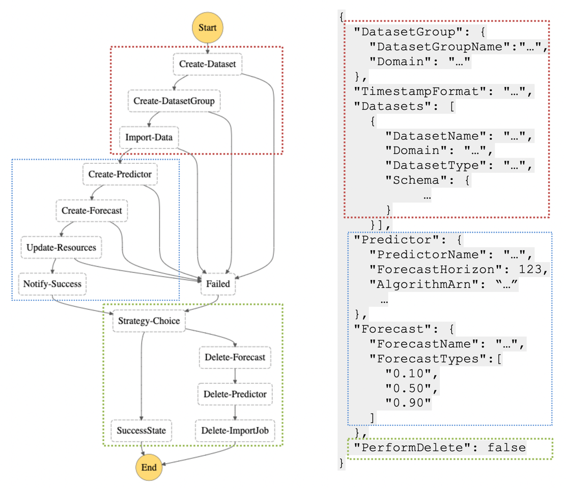
AWS Step Function steps example for an ML forecasting workflow

AWS has developed the Well-Architected Machine Learning Lens to help you review your operations and deployment, to determine whether or not you follow the best practices proposed by AWS. This approach utilizes security, operational efficiency, reliability, cost effectiveness, and performance. To keep your AI/ML operations robust, we highly recommend having these reviews internally and/or with your Solutions Architects or AWS Partners, regularly. Following Well-Architected best practices ensures that the MLOps process will reach its full potential for your organization.

Incorporating and interpreting AI/ML-based demand insights into the decision cycles

You can’t fully utilize the value of AI/ML without democratizing your insights. Setting business goals is an important step to success. Business goal should start with identification of a clear business objective. We recommend a measurable objective, because AI/ML will eventually utilize metrics for your organization. Continuously measure business value against specific business objectives and success criteria. Involve all stakeholders from the beginning to establish realistic but concrete value-delivering targets.

Once you determine your criteria for success, proceed with evaluating your organization's ability to move to the target. This includes the achievability of the objective, skill set, and tool set, as well as a clearly defined timeline for the objectives, which are regularly tracked and evaluated.

The business objective metric can easily be integrated into the Business Intelligence tool you use. In the previous chapter’s example for Amazon Forecast MLOps, you can build a dashboard for your business metrics in QuickSight. With QuickSight Q, your teams can ask questions about the results using natural communication, or use insights to your metrics.

If you prefer to use your own BI tool, you can still calculate custom metrics or use other types of queries using Amazon Athena views. The same process can be used with the SageMaker AI approach. You can use QuickSight with SageMaker AI through the relevant S3 bucket. Refer to the Visualizing Amazon SageMaker AI machine learning predictions with QuickSight blog post.

Example architectures

The following section shows two practical examples of demand forecasting for energy companies and GCP.

Energy forecasting example

The following diagram is an architecture for short-term electric demand forecasting that can be used for other demand forecasting use cases, as the concept is similar to other use cases. The proposed solution is using advanced Amazon Forecast features to solve forecasting problems. It is fully automated and event driven, with reduced manual processes. Also, it can scale as the forecasting needs increase.

Energy forecating architecture

The solution includes these broad steps:

• Module 1 - Ingest and transform data from the on-premises system 

• Module 2 - Forecast: Calling series of APIs to Amazon Forecast 

• Module 3 - Monitoring and notification

• Module 4 - Evaluation and visualization

The left box on the preceding diagram (labeled On-premises) is an example of field data ingestion that a typical utility has established on-premises. In this case, data ingestion from field sensors (a feeder head meter) is already in place through the PI System. Therefore, the starting point is raw circuit demand data extracted in Excel format, and stored on-premises. For Amazon Forecast to use this data, we first need to upload it to Amazon S3. This can be performed periodically by a scheduled script.

Next (in Module 1), as the raw data is available in Amazon S3 in utility custom-built formats, we need to massage the data. This involves extracting target data (consumption power in kilowatts), cleaning the data, and reformatting it. To do this, we use the services outlined in the box (labeled ETL and data lake) as follows:

• Amazon S3 is used to store raw and formatted data. This highly durable and highly available object storage is where the short-term electric load forecast (ST-ELF) input datasets will be consumed by Amazon Forecast.

• AWS Lambda is used to massage and transform the raw data. This serverless compute service runs your code in response to events (in this case, new raw file uploads) and automatically manages the computing resources required by the code.

• The Amazon Simple Queue Service (Amazon SQS), a fully managed message queuing service, decouples these transformation AWS Lambda functions. The queue acts as a buffer and can help smooth out traffic for the systems when consuming a multitude of events from many field sensors.

• AWS Glue is used for data cataloging, this service can run a crawler to update tables in your AWS AWS Glue Data Catalog, and as configured here, runs on a daily schedule.

• With data wrangling complete, the ST-ELF model is now ready for training. To train the model, we use Amazon Forecast (in Module 2). Using Amazon Forecast requires the import of training data, creation of a predictor (the ST-ELF model in this case), and creation of a forecast using the model, and finally exporting of the forecast and model accuracy metrics to Amazon S3.

• To streamline the process of ingesting, modeling and forecasting multiple ST-ELF models, the Improving Forecast Accuracy with Machine Learning solution is leveraged. This best practice AWS solution streamlines the process of ingesting, modeling, and forecasting using Amazon Forecast by providing AWS CloudFormation templates and a workflow around the Amazon Forecast service.

• Because forecasting might take some time to complete, the solution uses the Amazon Simple Notification Service (Amazon SNS) to send an email when the forecast is ready. Also, all AWS Lambda function logs are captured in Amazon CloudWatch (Module 3).

• Once the forecast is ready, the solution ensures your forecast data is ready and stored in Amazon S3. This fulfills a 14-day-ahead forecasting need. The solution also provides a mechanism to query the forecast input and output data with SQL using Amazon Athena (Module 4). Additionally, the solution can automatically create a visualization dashboard in the AWS Business Intelligence (BI) service QuickSight, which gives you the ability to visualize the data interactively in a dashboard.

Consumer Packaged Goods (CPG) forecasting example

This solution works with Amazon Vendor Central (sign-in required), but it can be used for other in-house or commercial endpoints. This solution builds a serverless architecture which is an event-based or scheduled pattern, that consistently and constantly pulls data from the CPG info endpoint into a persistent datastore. The data is then cataloged and analyzed through Amazon Athena, AWS Glue crawlers, and QuickSight. Here, Amazon purchase order (PO) data is ingested into Amazon Forecast to generate predictive analysis to help CPG companies improve on-time, in-full (OTIF) performance. To learn more about this solution, refer to CPG Companies: Improve Demand Forecasting to Boost Sales on Amazon.

Architecture to automate data collection for selling partners